課堂講義進度與 Griffiths 原文書(第5版)完全對照表
根據中原大學 1151 學年度電子三甲《電磁學(一)》授課大綱(課程代碼:EL214G,康振方副教授)及三份期中考投影片,精確映射至課本章節、定理與頁碼:
| 週次 | 講義 PDF 檔名 | 課堂教學單元 | Griffiths 5th Ed. 對應章節 | 課本頁碼 (Book / PDF) | 核心涵蓋概念與重點 |
|---|---|---|---|---|---|
| 第 1~5 週 | 電磁學(1)_1-向量分析.pdf 共 20 頁 |
第二章 向量分析:微分、積分形式、曲線座標、散度、旋度、斯托克定理 | Chapter 1: 1.1 ~ 1.4 Appendix A (Curvilinear) Appendix B (Helmholtz) |
pp. 1~56 (PDF pp. 27~82) 附錄: pp. 578~587 |
向量代數、三重積(BAC-CAB 展開)、尺度因子 $h_1, h_2, h_3$、梯度/散度/旋度/拉普拉斯算子之正交曲線座標推導、亥姆霍茲定理、馬克士威方程組物理意義。 |
| 第 6~8 週 | 電磁學(1)_2-Electrostatics.pdf 共 21 頁 |
第三章 靜電場:庫侖定律、連續電荷分佈、高斯定律、電位、帕松與拉普拉斯方程、靜電能量 | Chapter 2: 2.1 ~ 2.4 (2.1 Electric Field, 2.2 Gauss, 2.3 Potential, 2.4 Energy) |
pp. 57~95 (PDF pp. 83~121) |
庫侖定律與疊加原理、線段帶電體積分、高斯定律(球對稱、柱對稱、面對稱高斯面選取)、旋度 $\nabla\times\mathbf{E}=0$ 與保守場、電位定義與積分路徑、邊界條件不連續性、靜電位能兩種計算積分形式。 |
| 第 9 週 | 期中考試週 | 期中考試 (Midterm Exam) | Chap 1 ~ Chap 3 完整範圍 | 全體期中必考重點 | 評分比例 30%,著重向量推導、高斯定律應用、電位積分、鏡像法與分離變數法求解。 |
| 第 10~12 週 及進階延伸 |
電磁學(1)_3-Potentials.pdf 共 25 頁 |
第四章 靜電場問題:帕松及拉普拉斯方程、第一與第二唯一性定理、鏡像法、直交與球座標邊界值問題、多極展開 | Chapter 3: 3.1 ~ 3.4 (3.1 Laplace, 3.2 Images, 3.3 Separation, 3.4 Multipole) |
pp. 113~156 (PDF pp. 139~182) |
拉普拉斯方程之調和性質與平均值定理、唯一性定理、鏡像電荷(平面、接地球殼、不接地中性球殼、帶電球殼)、卡氏座標分離變數法(傅立葉級數正交性展開)、球座標分離變數法(勒壤得多項式 $P_l(\cos\theta)$)、電偶極勢與電場。 |
第一章 向量分析與正交曲線座標系 (Vector Analysis)
對應課本 Griffiths Chapter 1 (pp. 1~56) 及 Appendix A、B。包含正交曲線座標系尺度因子、基底變換與向量恆等式嚴格證明。
柱座標系統單位向量以直角座標(卡氏座標)表示
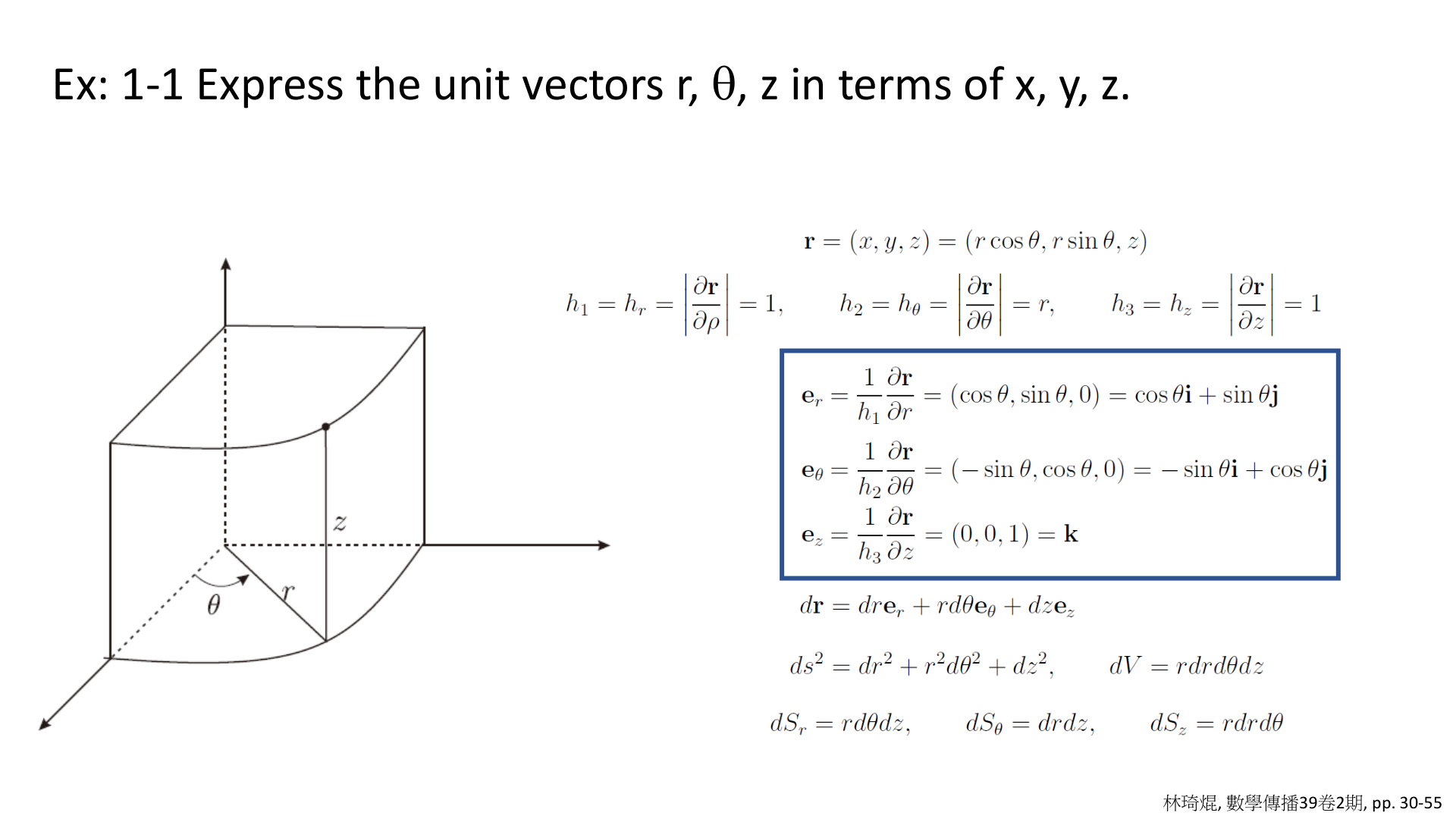
- 正交曲線座標幾何關係:柱座標 $(r, \theta, z)$ 與卡氏座標 $(x, y, z)$ 之轉化關係為 $x = r\cos\theta, y = r\sin\theta, z = z$。位置向量為 $\mathbf{r}(r, \theta, z) = x\mathbf{i} + y\mathbf{j} + z\mathbf{k} = r\cos\theta\,\mathbf{i} + r\sin\theta\,\mathbf{j} + z\mathbf{k}$。
- 度規尺度因子(Scale Factors):定義為切線向量之長度 $h_i = \left|\frac{\partial \mathbf{r}}{\partial q_i}\right|$。單位基底向量定義為 $\mathbf{e}_i = \frac{1}{h_i}\frac{\partial \mathbf{r}}{\partial q_i}$。
- 直交性驗證:$\mathbf{e}_r \cdot \mathbf{e}_\theta = 0, \mathbf{e}_r \cdot \mathbf{e}_z = 0, \mathbf{e}_\theta \cdot \mathbf{e}_z = 0$ 且 $\mathbf{e}_r \times \mathbf{e}_\theta = \mathbf{e}_z$ 構成右手正規正交基底。
在柱座標系統中,空間中任意點的位置向量 $\mathbf{r}$ 表為:
$$\mathbf{r} = (x, y, z) = (r\cos\theta, r\sin\theta, z) = r\cos\theta\,\mathbf{i} + r\sin\theta\,\mathbf{j} + z\mathbf{k}$$對各座標變數 $r, \theta, z$ 求偏導數:
$$\frac{\partial \mathbf{r}}{\partial r} = \cos\theta\,\mathbf{i} + \sin\theta\,\mathbf{j} + 0\mathbf{k} = (\cos\theta, \sin\theta, 0)$$ $$\frac{\partial \mathbf{r}}{\partial \theta} = -r\sin\theta\,\mathbf{i} + r\cos\theta\,\mathbf{j} + 0\mathbf{k} = (-r\sin\theta, r\cos\theta, 0)$$ $$\frac{\partial \mathbf{r}}{\partial z} = 0\mathbf{i} + 0\mathbf{j} + 1\mathbf{k} = (0, 0, 1)$$取各偏導數向量之歐幾里得範數(長度):
$$h_1 = h_r = \left|\frac{\partial \mathbf{r}}{\partial r}\right| = \sqrt{\cos^2\theta + \sin^2\theta + 0} = 1$$ $$h_2 = h_\theta = \left|\frac{\partial \mathbf{r}}{\partial \theta}\right| = \sqrt{(-r\sin\theta)^2 + (r\cos\theta)^2 + 0} = \sqrt{r^2(\sin^2\theta + \cos^2\theta)} = r$$ $$h_3 = h_z = \left|\frac{\partial \mathbf{r}}{\partial z}\right| = \sqrt{0^2 + 0^2 + 1^2} = 1$$利用公式 $\mathbf{e}_i = \frac{1}{h_i}\frac{\partial \mathbf{r}}{\partial q_i}$:
以矩陣形式表示轉化關係為:
$$\begin{bmatrix} \mathbf{e}_r \\ \mathbf{e}_\theta \\ \mathbf{e}_z \end{bmatrix} = \begin{bmatrix} \cos\theta & \sin\theta & 0 \\ -\sin\theta & \cos\theta & 0 \\ 0 & 0 & 1 \end{bmatrix} \begin{bmatrix} \mathbf{i} \\ \mathbf{j} \\ \mathbf{k} \end{bmatrix}$$全微分弧長向量 $d\mathbf{r}$ 為:
$$d\mathbf{r} = h_r dr\,\mathbf{e}_r + h_\theta d\theta\,\mathbf{e}_\theta + h_z dz\,\mathbf{e}_z = dr\,\mathbf{e}_r + r d\theta\,\mathbf{e}_\theta + dz\,\mathbf{e}_z$$微分線元素平方度規(Line element squared):
$$ds^2 = |d\mathbf{r}|^2 = dr^2 + r^2 d\theta^2 + dz^2$$三方向之微分面積元(Area elements):
$$dS_r = (h_\theta d\theta)(h_z dz) = r\,d\theta\,dz$$ $$dS_\theta = (h_r dr)(h_z dz) = dr\,dz$$ $$dS_z = (h_r dr)(h_\theta d\theta) = r\,dr\,d\theta$$微分體積元(Volume element):
球座標系統單位向量以直角座標表示與尺度因子推導
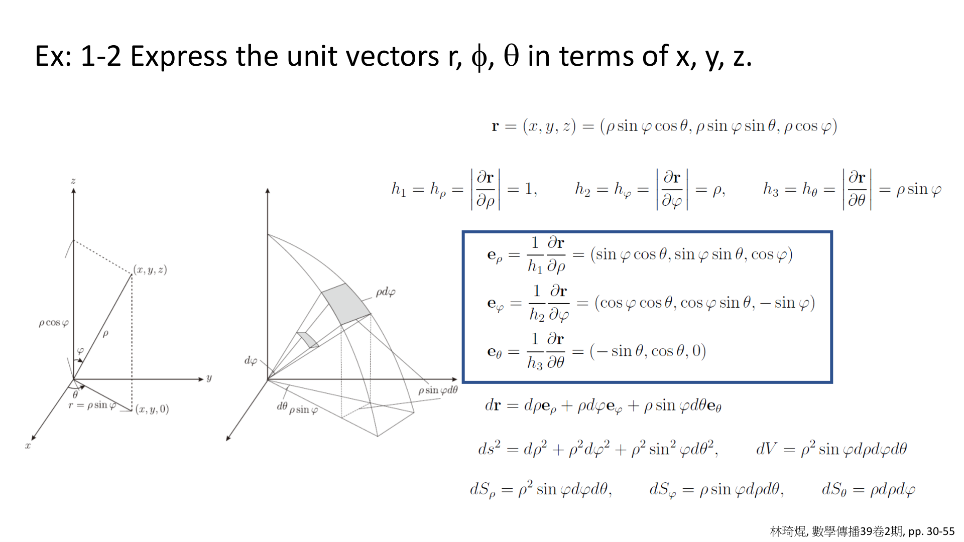
- 座標定義注意:講義採林琦焜教授文獻符號:$\rho$ 為半徑(即物理上之 $r$),$\phi$ 為與 $z$ 軸夾角(即物理上之天頂角 $\theta$),$\theta$ 為 $xy$ 平面上之方位角(即物理上之 $\phi$)。
- 卡氏轉換關係:$x = \rho\sin\phi\cos\theta,\; y = \rho\sin\phi\sin\theta,\; z = \rho\cos\phi$。
- 切線度規本質:$h_i$ 代表當該座標變數增加 $dq_i$ 時,空間實際位移的大小。由於 $\phi$ 與 $\theta$ 為無因次弧度,其尺度因子必帶有長度因次。
將位置向量寫為三維卡氏分量:
$$\mathbf{r}(\rho, \phi, \theta) = (\rho\sin\phi\cos\theta)\mathbf{i} + (\rho\sin\phi\sin\theta)\mathbf{j} + (\rho\cos\phi)\mathbf{k}$$分別對 $\rho, \phi, \theta$ 求一階偏導微商:
$$\frac{\partial \mathbf{r}}{\partial \rho} = \sin\phi\cos\theta\,\mathbf{i} + \sin\phi\sin\theta\,\mathbf{j} + \cos\phi\,\mathbf{k}$$ $$\frac{\partial \mathbf{r}}{\partial \phi} = \rho\cos\phi\cos\theta\,\mathbf{i} + \rho\cos\phi\sin\theta\,\mathbf{j} - \rho\sin\phi\,\mathbf{k}$$ $$\frac{\partial \mathbf{r}}{\partial \theta} = -\rho\sin\phi\sin\theta\,\mathbf{i} + \rho\sin\phi\cos\theta\,\mathbf{j} + 0\mathbf{k}$$計算各微商向量之範數長度:
$$h_\rho = \left|\frac{\partial \mathbf{r}}{\partial \rho}\right| = \sqrt{\sin^2\phi(\cos^2\theta + \sin^2\theta) + \cos^2\phi} = \sqrt{\sin^2\phi + \cos^2\phi} = 1$$ $$h_\phi = \left|\frac{\partial \mathbf{r}}{\partial \phi}\right| = \sqrt{\rho^2\cos^2\phi(\cos^2\theta + \sin^2\theta) + \rho^2\sin^2\phi} = \sqrt{\rho^2(\cos^2\phi + \sin^2\phi)} = \rho$$ $$h_\theta = \left|\frac{\partial \mathbf{r}}{\partial \theta}\right| = \sqrt{\rho^2\sin^2\phi(\sin^2\theta + \cos^2\theta)} = \rho\sin\phi$$將微商向量除以對應之尺度因子即可得正規正交單位向量:
轉化矩陣為正交矩陣(Orthogonal Matrix,逆矩陣即轉置矩陣):
$$\begin{bmatrix} \mathbf{e}_\rho \\ \mathbf{e}_\phi \\ \mathbf{e}_\theta \end{bmatrix} = \begin{bmatrix} \sin\phi\cos\theta & \sin\phi\sin\theta & \cos\phi \\ \cos\phi\cos\theta & \cos\phi\sin\theta & -\sin\phi \\ -\sin\theta & \cos\theta & 0 \end{bmatrix} \begin{bmatrix} \mathbf{i} \\ \mathbf{j} \\ \mathbf{k} \end{bmatrix}$$位移向量微分:
$$d\mathbf{r} = d\rho\,\mathbf{e}_\rho + \rho\,d\phi\,\mathbf{e}_\phi + \rho\sin\phi\,d\theta\,\mathbf{e}_\theta$$線元素平方度規:
$$ds^2 = d\rho^2 + \rho^2 d\phi^2 + \rho^2\sin^2\phi\,d\theta^2$$面積微元:
$$dS_\rho = (h_\phi d\phi)(h_\theta d\theta) = \rho^2\sin\phi\,d\phi\,d\theta$$ $$dS_\phi = (h_\rho d\rho)(h_\theta d\theta) = \rho\sin\phi\,d\rho\,d\theta$$ $$dS_\theta = (h_\rho d\rho)(h_\phi d\phi) = \rho\,d\rho\,d\phi$$體積微元(Griffiths 記為 $d\tau = r^2\sin\theta\,dr\,d\theta\,d\phi$):
向量三重積 BAC-CAB 公式之幾何與代數嚴密證明
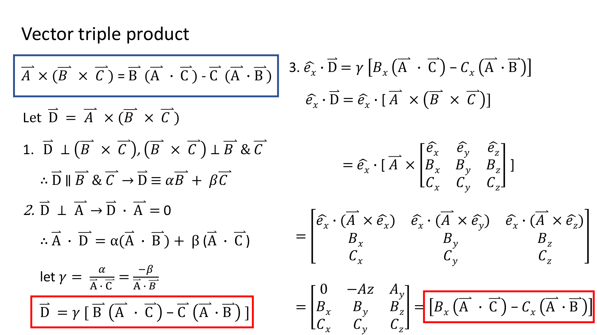
令向量 $\mathbf{D} \equiv \mathbf{A} \times (\mathbf{B} \times \mathbf{C})$。
1. 根據外積定義,$\mathbf{D}$ 必垂直於向量 $(\mathbf{B} \times \mathbf{C})$。而 $(\mathbf{B} \times \mathbf{C})$ 垂直於 $\mathbf{B}$ 與 $\mathbf{C}$ 所在的平面。因此,$\mathbf{D}$ 必然平行(共面)於 $\mathbf{B}$ 與 $\mathbf{C}$ 所張成的平面!
故 $\mathbf{D}$ 必可表示為 $\mathbf{B}$ 與 $\mathbf{C}$ 的線性組合:
$$\mathbf{D} = \alpha \mathbf{B} + \beta \mathbf{C}$$2. 同時,$\mathbf{D}$ 來自 $\mathbf{A} \times (\dots)$,故 $\mathbf{D}$ 必定與 $\mathbf{A}$ 正交垂直:
$$\mathbf{A} \cdot \mathbf{D} = 0$$將 $\mathbf{D} = \alpha \mathbf{B} + \beta \mathbf{C}$ 代入點積式:
$$\mathbf{A} \cdot (\alpha \mathbf{B} + \beta \mathbf{C}) = \alpha (\mathbf{A} \cdot \mathbf{B}) + \beta (\mathbf{A} \cdot \mathbf{C}) = 0$$移項得係數關係式:
$$\frac{\alpha}{\mathbf{A} \cdot \mathbf{C}} = \frac{-\beta}{\mathbf{A} \cdot \mathbf{B}} \equiv \gamma$$其中 $\gamma$ 為某一純量待定常數。因此:
$$\alpha = \gamma (\mathbf{A} \cdot \mathbf{C}), \quad \beta = -\gamma (\mathbf{A} \cdot \mathbf{B})$$ $$\mathbf{D} = \gamma \left[ \mathbf{B}(\mathbf{A} \cdot \mathbf{C}) - \mathbf{C}(\mathbf{A} \cdot \mathbf{B}) \right]$$取 $\mathbf{e}_x \cdot \mathbf{D} = D_x$。右側展開:
$$D_x = \gamma \left[ B_x (\mathbf{A} \cdot \mathbf{C}) - C_x (\mathbf{A} \cdot \mathbf{B}) \right]$$另一方面,直接計算三重積的 $x$ 分量:
$$D_x = \mathbf{e}_x \cdot [\mathbf{A} \times (\mathbf{B} \times \mathbf{C})] = (\mathbf{e}_x \times \mathbf{A}) \cdot (\mathbf{B} \times \mathbf{C})$$利用純量三重積行列式計算:
$$\mathbf{e}_x \cdot [\mathbf{A} \times (\mathbf{B} \times \mathbf{C})] = \begin{vmatrix} 0 & -A_z & A_y \\ B_x & B_y & B_z \\ C_x & C_y & C_z \end{vmatrix} = A_z(B_x C_z - B_z C_x) + A_y(B_x C_y - B_y C_x)$$重組項次:
$$= B_x(A_y C_y + A_z C_z) - C_x(A_y B_y + A_z B_z)$$在兩括號內分別補上 $A_x C_x B_x$ 與相減項:
$$= B_x (A_x C_x + A_y C_y + A_z C_z) - C_x (A_x B_x + A_y B_y + A_z B_z) = B_x (\mathbf{A} \cdot \mathbf{C}) - C_x (\mathbf{A} \cdot \mathbf{B})$$兩式對比,得證比例常數 $\gamma = 1$!
向量場散度 (Divergence) 與旋度 (Curl) 基本運算與無旋場判別


(a) $\mathbf{v}_a = x^2\hat{\mathbf{x}} + 3xz^2\hat{\mathbf{y}} - 2xz\hat{\mathbf{z}}$
(b) $\mathbf{v}_b = xy\hat{\mathbf{x}} + 2yz\hat{\mathbf{y}} + 3zx\hat{\mathbf{z}}$
(c) $\mathbf{v}_c = y^2\hat{\mathbf{x}} + (2xy + z^2)\hat{\mathbf{y}} + 2yz\hat{\mathbf{z}}$
Problem 1.18: Calculate the curls of the vector functions in Prob. 1.15.
散度計算:
$$\nabla \cdot \mathbf{v}_a = \frac{\partial (x^2)}{\partial x} + \frac{\partial (3xz^2)}{\partial y} + \frac{\partial (-2xz)}{\partial z} = 2x + 0 - 2x = 0$$此向量場為螺線場(Solenoidal Field),散度處處為 0。
旋度計算:
$$\nabla \times \mathbf{v}_a = \begin{vmatrix} \hat{\mathbf{x}} & \hat{\mathbf{y}} & \hat{\mathbf{z}} \\ \frac{\partial}{\partial x} & \frac{\partial}{\partial y} & \frac{\partial}{\partial z} \\ x^2 & 3xz^2 & -2xz \end{vmatrix} = \hat{\mathbf{x}}(0 - 6xz) - \hat{\mathbf{y}}(-2z - 0) + \hat{\mathbf{z}}(3z^2 - 0)$$散度計算:
$$\nabla \cdot \mathbf{v}_b = \frac{\partial (xy)}{\partial x} + \frac{\partial (2yz)}{\partial y} + \frac{\partial (3zx)}{\partial z} = y + 2z + 3x$$旋度計算:
$$\nabla \times \mathbf{v}_b = \begin{vmatrix} \hat{\mathbf{x}} & \hat{\mathbf{y}} & \hat{\mathbf{z}} \\ \frac{\partial}{\partial x} & \frac{\partial}{\partial y} & \frac{\partial}{\partial z} \\ xy & 2yz & 3zx \end{vmatrix} = \hat{\mathbf{x}}(0 - 2y) - \hat{\mathbf{y}}(3z - 0) + \hat{\mathbf{z}}(0 - x)$$散度計算:
$$\nabla \cdot \mathbf{v}_c = \frac{\partial (y^2)}{\partial x} + \frac{\partial (2xy + z^2)}{\partial y} + \frac{\partial (2yz)}{\partial z} = 0 + 2x + 2y = 2(x + y)$$旋度計算:
$$\nabla \times \mathbf{v}_c = \begin{vmatrix} \hat{\mathbf{x}} & \hat{\mathbf{y}} & \hat{\mathbf{z}} \\ \frac{\partial}{\partial x} & \frac{\partial}{\partial y} & \frac{\partial}{\partial z} \\ y^2 & 2xy+z^2 & 2yz \end{vmatrix} = \hat{\mathbf{x}}(2z - 2z) - \hat{\mathbf{y}}(0 - 0) + \hat{\mathbf{z}}(2y - 2y) = \mathbf{0}$$物理重點:$\mathbf{v}_c$ 旋度處處為零,為無旋場(Irrotational Field),必可寫為某純量勢之梯度:$\mathbf{v}_c = \nabla (x y^2 + y z^2)$!
高斯散度定理(Divergence Theorem)之立體驗證
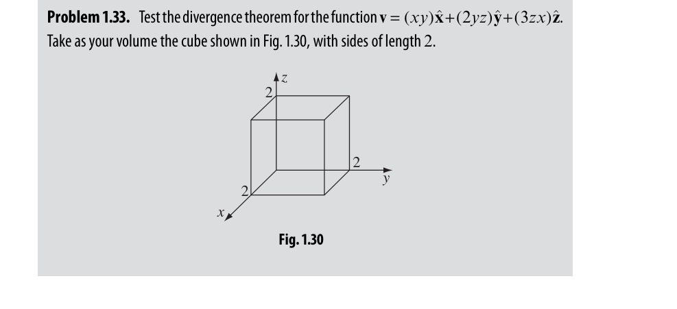
先求散度:
$$\nabla \cdot \mathbf{v} = \frac{\partial (xy)}{\partial x} + \frac{\partial (2yz)}{\partial y} + \frac{\partial (3zx)}{\partial z} = y + 2z + 3x$$在單位立方體 $x, y, z \in [0, 1]$ 內進行三重體積分:
$$\int_V (\nabla \cdot \mathbf{v}) d\tau = \int_0^1 dx \int_0^1 dy \int_0^1 dz\,(3x + y + 2z)$$ $$= \int_0^1 3x\,dx \cdot (1)(1) + \int_0^1 y\,dy \cdot (1)(1) + \int_0^1 2z\,dz \cdot (1)(1)$$ $$= \frac{3}{2} + \frac{1}{2} + 1 = 3$$- 面 1 ($x = 1$, $d\mathbf{a} = dy dz\,\hat{\mathbf{x}}$):$\mathbf{v}\cdot d\mathbf{a} = (1\cdot y) dy dz \implies \int_0^1 \int_0^1 y\,dy dz = \frac{1}{2}$
- 面 2 ($x = 0$, $d\mathbf{a} = -dy dz\,\hat{\mathbf{x}}$):$\mathbf{v}\cdot d\mathbf{a} = -(0\cdot y) dy dz = 0$
- 面 3 ($y = 1$, $d\mathbf{a} = dx dz\,\hat{\mathbf{y}}$):$\mathbf{v}\cdot d\mathbf{a} = (2\cdot 1\cdot z) dx dz \implies \int_0^1 \int_0^1 2z\,dx dz = 1$
- 面 4 ($y = 0$, $d\mathbf{a} = -dx dz\,\hat{\mathbf{y}}$):$\mathbf{v}\cdot d\mathbf{a} = -(2\cdot 0\cdot z) dx dz = 0$
- 面 5 ($z = 1$, $d\mathbf{a} = dx dy\,\hat{\mathbf{z}}$):$\mathbf{v}\cdot d\mathbf{a} = (3\cdot 1\cdot x) dx dy \implies \int_0^1 \int_0^1 3x\,dx dy = \frac{3}{2}$
- 面 6 ($z = 0$, $d\mathbf{a} = -dx dy\,\hat{\mathbf{z}}$):$\mathbf{v}\cdot d\mathbf{a} = -(3\cdot 0\cdot x) dx dy = 0$
將六個面的表面通量相加:
$$\oint_S \mathbf{v} \cdot d\mathbf{a} = \frac{1}{2} + 0 + 1 + 0 + \frac{3}{2} + 0 = 3$$體積分與閉曲面積分結果完全相等,散度定理得證!
第二章 靜電學:電場、高斯定律、電位與靜電能量 (Electrostatics)
對應課本 Griffiths Chapter 2 (pp. 57~112)。涵蓋庫侖定律、連續電荷分佈積分、高斯定律三大對稱應用、電位積分、帕松方程與靜電能量計算。
兩同性點電荷中垂線上方之電場求解與遠距極限
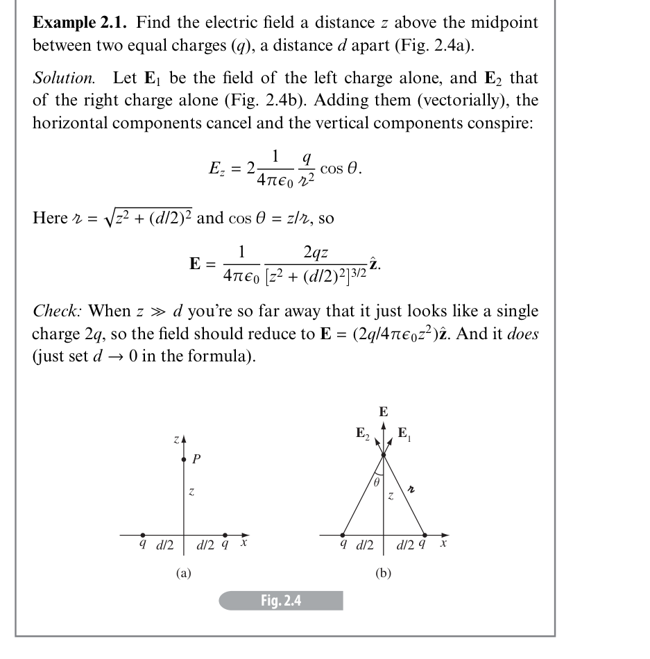
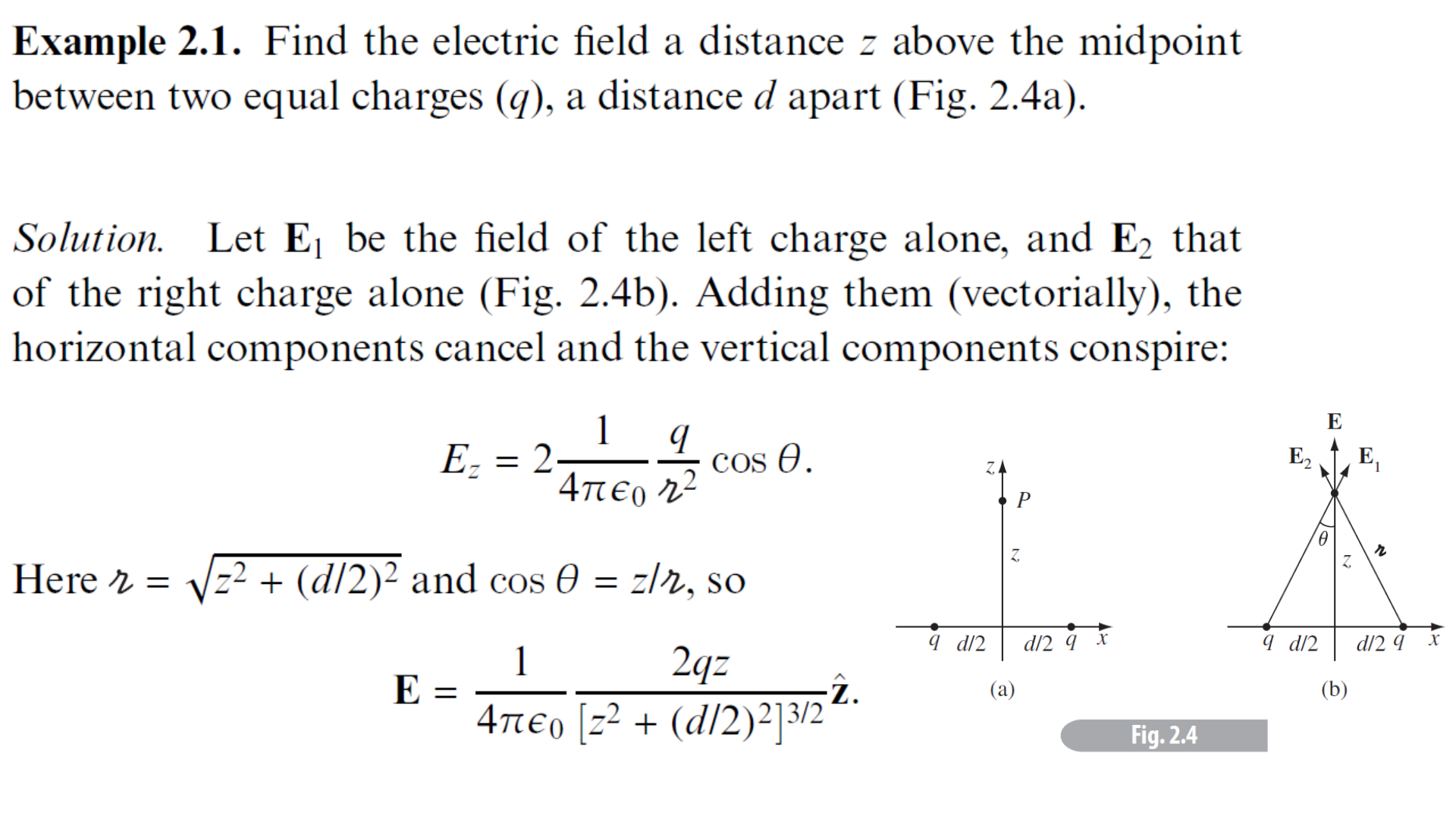
- 庫侖定律 (Coulomb's Law):單一電荷在場點產生的電場為 $\mathbf{E} = \frac{1}{4\pi\epsilon_0}\frac{q}{r^2}\hat{\boldsymbol{r}}$。
- 對稱性抵消 (Symmetry Cancellation):由於兩正電荷大小相等且對稱位於 $x = \pm d/2$,兩電荷在場點產生的水平水平($x$ 方向)分量大小相等、方向相反互相完全抵消;垂直垂直($z$ 方向)分量同向共謀相加。
將左側電荷置於 $(-d/2, 0, 0)$,右側電荷置於 $(+d/2, 0, 0)$,場點 $P$ 位於 $(0, 0, z)$。
任一電荷到場點的直線距離(分離距離 $r$)均為:
$$r = \sqrt{z^2 + (d/2)^2}$$電場與 $z$ 軸夾角為 $\theta$,由直角三角形幾何得方向餘弦:
$$\cos\theta = \frac{z}{r} = \frac{z}{\sqrt{z^2 + (d/2)^2}}$$水平分量:$E_x = E_{1x} + E_{2x} = -E_1\sin\theta + E_2\sin\theta = 0$。
垂直分量兩者同向疊加:
$$E_z = 2 E_1 \cos\theta = 2 \left( \frac{1}{4\pi\epsilon_0}\frac{q}{r^2} \right) \cos\theta = 2 \left( \frac{1}{4\pi\epsilon_0}\frac{q}{z^2 + (d/2)^2} \right) \frac{z}{\sqrt{z^2 + (d/2)^2}}$$兩異性電荷(電偶極)中垂線上方之電場與偶極極限
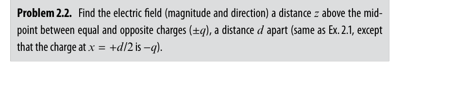
設 $+q$ 位於 $(-d/2, 0, 0)$,$-q$ 位於 $(+d/2, 0, 0)$。場點為 $(0, 0, z)$。
$+q$ 產生之電場 $\mathbf{E}_+$ 指向遠離 $+q$ 之方向;$-q$ 產生之電場 $\mathbf{E}_-$ 指向 $-q$。
由幾何對稱可知:兩者在垂直方向($z$ 方向)的大小相等、方向相反($+q$ 向上推、$-q$ 向下拉),因而 $z$ 分量完全抵消!
反之,在水平方向(沿 $+x$ 軸方向),兩者的水平分量同向疊加:
$$\sin\theta = \frac{d/2}{r} = \frac{d/2}{\sqrt{z^2 + (d/2)^2}}$$水平合電場大小為:
$$E_x = E_+ \sin\theta + E_- \sin\theta = 2 \left( \frac{1}{4\pi\epsilon_0} \frac{q}{r^2} \right) \sin\theta$$ $$E_x = 2 \left( \frac{1}{4\pi\epsilon_0} \frac{q}{z^2 + (d/2)^2} \right) \frac{d/2}{\sqrt{z^2 + (d/2)^2}} = \frac{1}{4\pi\epsilon_0} \frac{qd}{\left[ z^2 + (d/2)^2 \right]^{3/2}}$$方向朝向 $+x$ 軸方向(從正電荷指向負電荷之反方向):
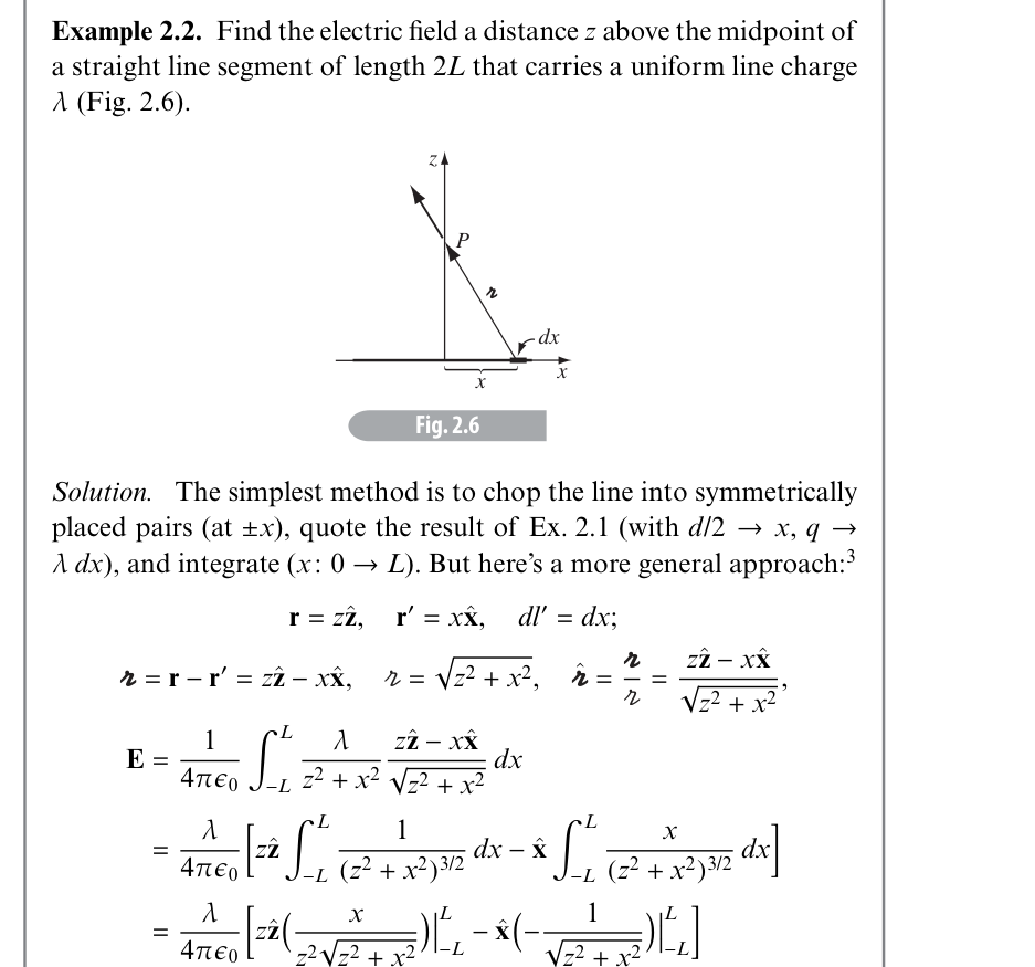
有限長均勻帶電線段之中垂線電場與極限討論 (1) $z\to\infty$ (2) $L\to\infty$
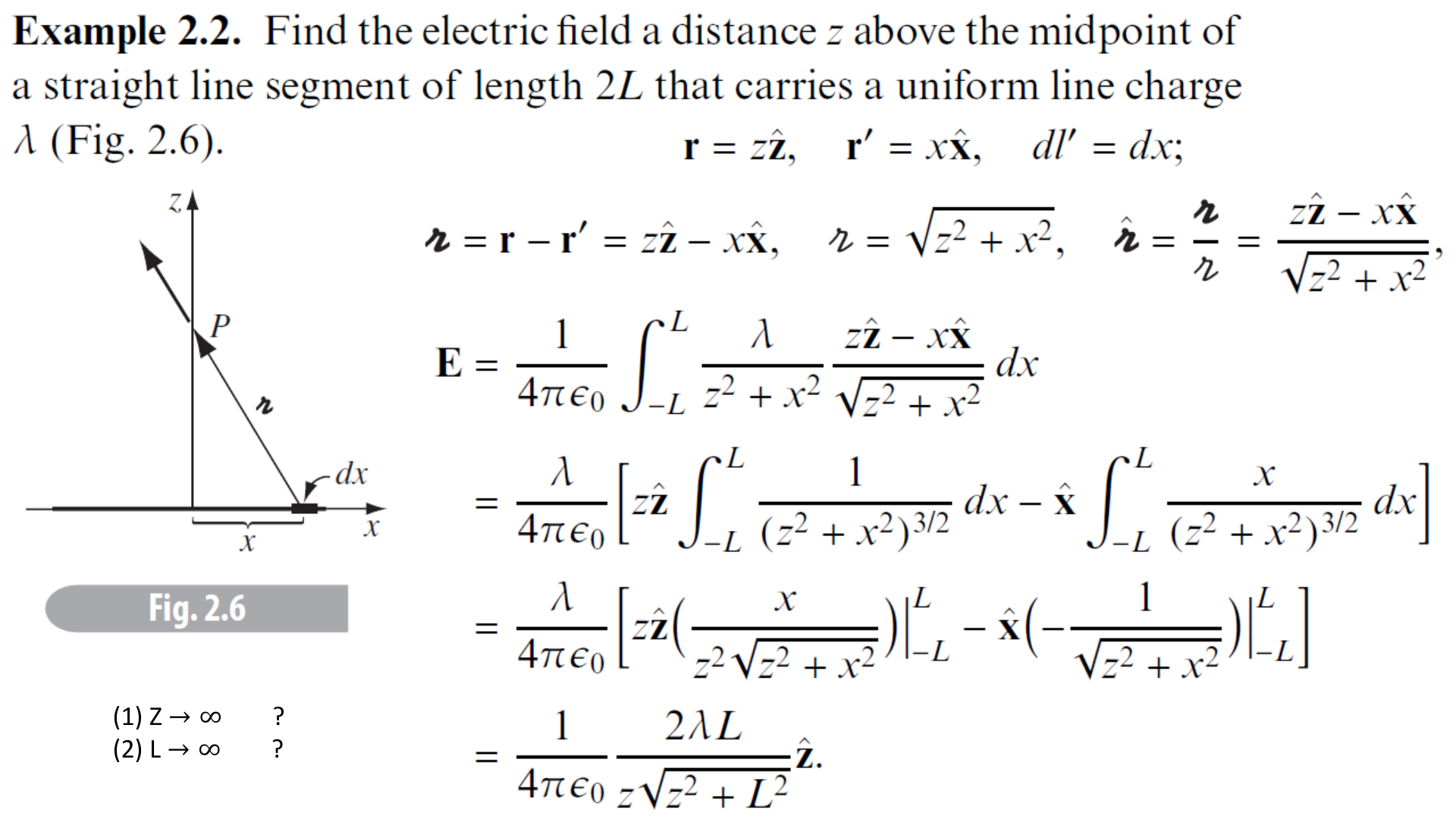
Lecture Slide Follow-up Questions:
(1) What is $\mathbf{E}$ as $z \to \infty$?
(2) What is $\mathbf{E}$ as $L \to \infty$?
講義補充指定思考題:
(1) 當 $z \to \infty$(距離極遠)時,電場為何?
(2) 當 $L \to \infty$(無限長帶電直線)時,電場為何?
將帶電線段置於 $x$ 軸上,範圍從 $x = -L$ 到 $x = +L$。中點位於原點。場點為 $(0, 0, z)$。
線段上一微小線元 $dl' = dx$,其位置向量為 $\mathbf{r}' = x\hat{\mathbf{x}}$。場點位置向量為 $\mathbf{r} = z\hat{\mathbf{z}}$。
分離向量(Separation vector):
$$\boldsymbol{r} = \mathbf{r} - \mathbf{r}' = z\hat{\mathbf{z}} - x\hat{\mathbf{x}}, \quad r = |\boldsymbol{r}| = \sqrt{z^2 + x^2}, \quad \hat{\boldsymbol{r}} = \frac{z\hat{\mathbf{z}} - x\hat{\mathbf{x}}}{\sqrt{z^2 + x^2}}$$電荷微元為 $dq = \lambda dx$。
根據連續電荷庫侖定律:
$$\mathbf{E} = \frac{1}{4\pi\epsilon_0} \int_{-L}^L \frac{\lambda dx}{r^2}\hat{\boldsymbol{r}} = \frac{1}{4\pi\epsilon_0} \int_{-L}^L \frac{\lambda(z\hat{\mathbf{z}} - x\hat{\mathbf{x}})}{(z^2 + x^2)^{3/2}} dx$$拆解為 $x$ 與 $z$ 兩部分:
$$\mathbf{E} = \frac{\lambda}{4\pi\epsilon_0} \left[ z\hat{\mathbf{z}} \int_{-L}^L \frac{dx}{(z^2 + x^2)^{3/2}} - \hat{\mathbf{x}} \int_{-L}^L \frac{x dx}{(z^2 + x^2)^{3/2}} \right]$$注意第二項被積函數 $\frac{x}{(z^2 + x^2)^{3/2}}$ 為關於 $x$ 的奇函數(Odd function),在對稱區間 $[-L, L]$ 上之定積分為零:
$$\int_{-L}^L \frac{x dx}{(z^2 + x^2)^{3/2}} = 0$$故水平分量因對稱性完全抵消,僅存 $z$ 方向分量!
利用標準積分公式 $\int \frac{dx}{(z^2 + x^2)^{3/2}} = \frac{x}{z^2 \sqrt{z^2 + x^2}}$:
$$\int_{-L}^L \frac{dx}{(z^2 + x^2)^{3/2}} = \left. \frac{x}{z^2 \sqrt{z^2 + x^2}} \right|_{-L}^L = \frac{L}{z^2 \sqrt{z^2 + L^2}} - \left( \frac{-L}{z^2 \sqrt{z^2 + L^2}} \right) = \frac{2L}{z^2 \sqrt{z^2 + L^2}}$$代入電場表達式:
問題 (1):當 $z \to \infty$(場點遠離線段)?
當 $z \gg L$ 時,$\sqrt{z^2 + L^2} = z\sqrt{1 + (L/z)^2} \approx z$。代入得:
$$\mathbf{E} \approx \frac{1}{4\pi\epsilon_0} \frac{2\lambda L}{z(z)} \hat{\mathbf{z}} = \frac{1}{4\pi\epsilon_0} \frac{q_{\text{total}}}{z^2} \hat{\mathbf{z}}$$其中 $q_{\text{total}} = 2\lambda L$ 為整個線段的總電荷。此結果表明:當觀察者距離極遠時,有限長度的線電荷縮為一個點,電場退化為標準點電荷平方反比場!
問題 (2):當 $L \to \infty$(線段長度趨於無窮大,無限長直導線)?
當 $L \gg z$ 時,$\sqrt{z^2 + L^2} = L\sqrt{1 + (z/L)^2} \approx L$。代入得:
$$\mathbf{E} = \frac{1}{4\pi\epsilon_0} \frac{2\lambda L}{z(L)} \hat{\mathbf{z}} = \frac{1}{4\pi\epsilon_0} \frac{2\lambda}{z} \hat{\mathbf{z}} = \frac{\lambda}{2\pi\epsilon_0 z} \hat{\mathbf{z}}$$此即無限長均勻帶電直線所產生的徑向電場公式(稍後將用高斯定律在數秒內再次導出),電場以 $1/z$ 衰減!
高斯定律求解均勻帶電實心球體之內部與外部電場
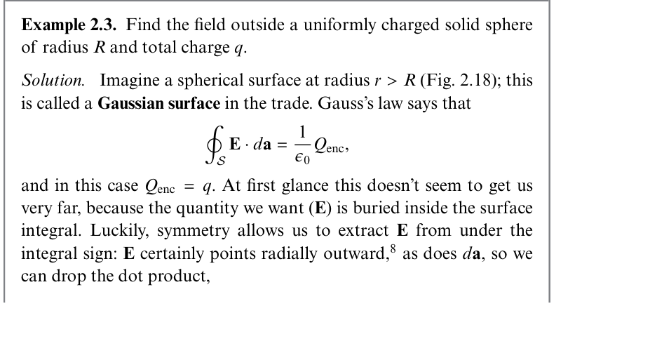
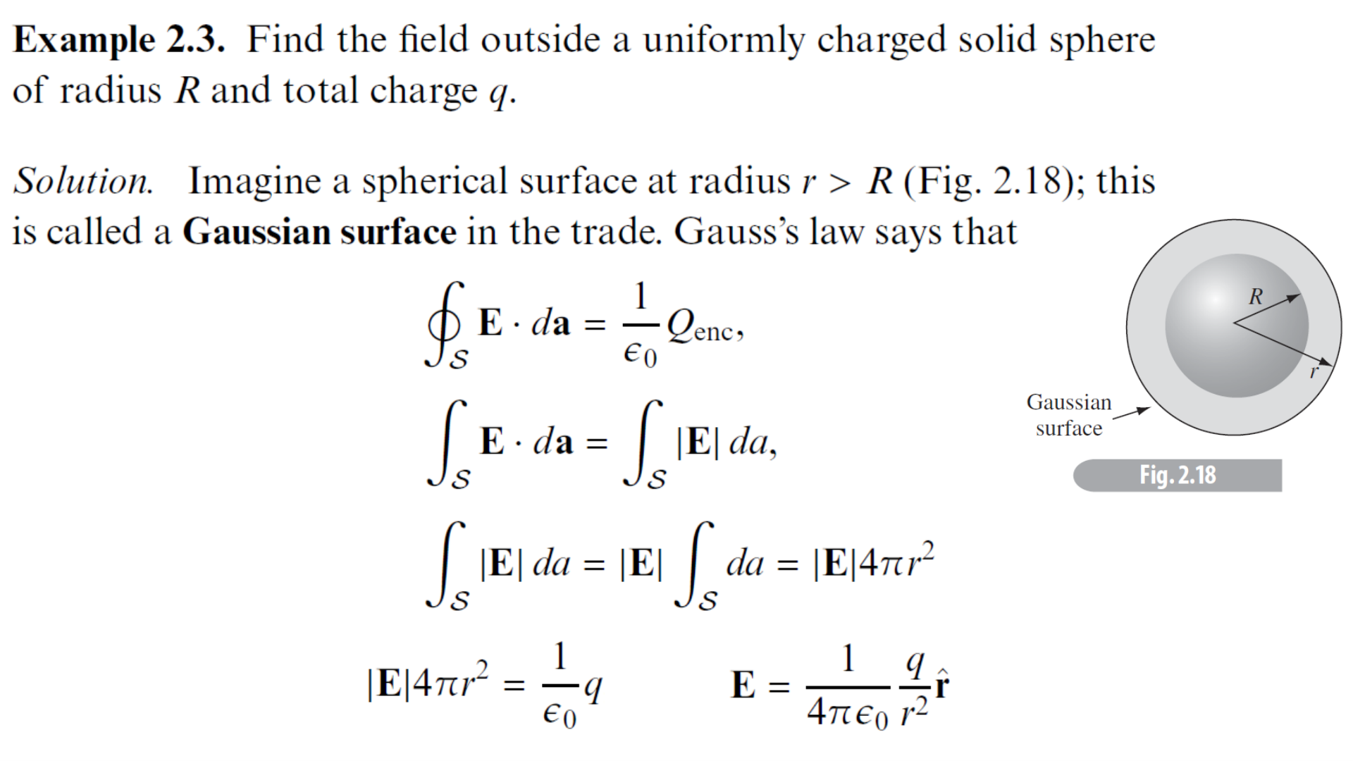
Problem 2.13 (Inside Field): Use Gauss's law to find the electric field inside a uniformly charged solid sphere ($r < R$).
電荷分佈具有完美的球對稱性(Spherical Symmetry)。因此電場只能沿徑向,且大小僅取決於與球心的距離 $r$:
$$\mathbf{E} = E(r)\hat{\mathbf{r}}$$選取半徑為 $r$、以球心為中心的同心球面作為高斯面 $S$。在該面上,面元向量 $d\mathbf{a} = da\,\hat{\mathbf{r}}$ 處處與 $\mathbf{E}$ 平行:
$$\oint_S \mathbf{E} \cdot d\mathbf{a} = \oint_S E(r)\,da = E(r) \oint_S da = E(r) (4\pi r^2)$$根據高斯定律,該通量恆等於 $\frac{1}{\epsilon_0} Q_{\text{enc}}$:
$$E(r) (4\pi r^2) = \frac{Q_{\text{enc}}}{\epsilon_0} \implies E(r) = \frac{1}{4\pi\epsilon_0} \frac{Q_{\text{enc}}}{r^2}$$高斯面完全包覆整個實心球體,故內部包覆電荷即為總電荷:
$$Q_{\text{enc}} = q$$外部電場與所有電荷集中在球心的點電荷場完全一致。
半徑為 $r$ 的內部高斯面包覆之體積為 $\frac{4}{3}\pi r^3$。所包含的電荷為體積比值:
$$Q_{\text{enc}} = \rho \left( \frac{4}{3}\pi r^3 \right) = \left( \frac{q}{\frac{4}{3}\pi R^3} \right) \left( \frac{4}{3}\pi r^3 \right) = q \left( \frac{r}{R} \right)^3$$代入高斯定律:
$$E(r) (4\pi r^2) = \frac{1}{\epsilon_0} q \frac{r^3}{R^3} \implies E(r) = \frac{1}{4\pi\epsilon_0} \frac{q r}{R^3}$$內部電場隨半徑 $r$ 線性增長,在球心 $r=0$ 處為零,在表面 $r=R$ 處與外部解連續相接!
非均勻電荷密度長圓柱之內部電場(高斯定律柱對稱)
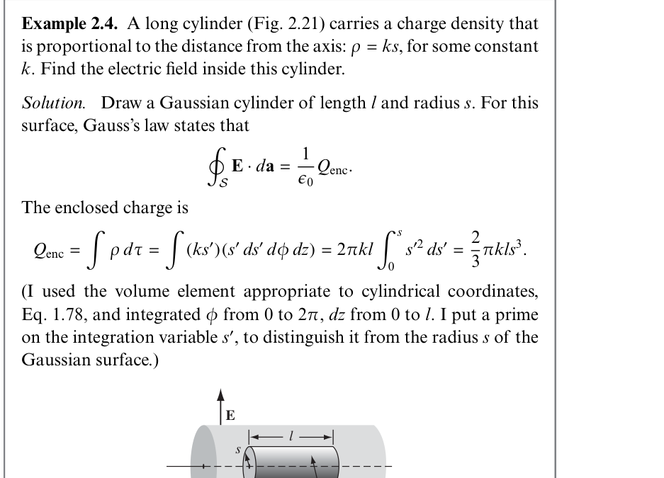
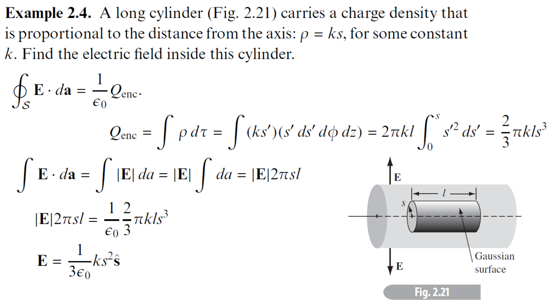
系統具有無限長柱對稱性(Cylindrical Symmetry)。電場方向必沿徑向 $\hat{\mathbf{s}}$,且大小僅為 $s$ 的函數:$\mathbf{E} = E(s)\hat{\mathbf{s}}$。
在圓柱體內部選取同軸的高斯圓柱面:半徑為 $s$,長度為 $l$。
該閉合高斯面由三部分組成:兩個端面圓盤與一個側表面。
- 兩端面:法向量沿 $\pm\hat{\mathbf{z}}$,與電場 $\mathbf{E} \parallel \hat{\mathbf{s}}$ 垂直,故端面通量為零:$\int_{\text{ends}} \mathbf{E} \cdot d\mathbf{a} = 0$。
- 圓柱側表面:法向量處處沿 $\hat{\mathbf{s}}$,電場大小為常數 $E(s)$:
利用柱座標體積元 $d\tau = s' ds' d\phi dz$ 對電荷密度進行體積分:
$$Q_{\text{enc}} = \int \rho\,d\tau = \int_0^l dz \int_0^{2\pi} d\phi \int_0^s (k s')(s' ds') = (l)(2\pi) k \int_0^s (s')^2 ds'$$ $$Q_{\text{enc}} = 2\pi k l \left[ \frac{(s')^3}{3} \right]_0^s = \frac{2}{3}\pi k l s^3$$高斯定律公式:$\oint \mathbf{E} \cdot d\mathbf{a} = \frac{Q_{\text{enc}}}{\epsilon_0}$
$$|E|(2\pi s l) = \frac{1}{\epsilon_0} \left( \frac{2}{3}\pi k l s^3 \right)$$消去兩側公因式 $2\pi l s$:
電場與半徑平方 $s^2$ 成正比,方向徑向向外。
無限大均勻帶電平面與無限長帶電直線之電場
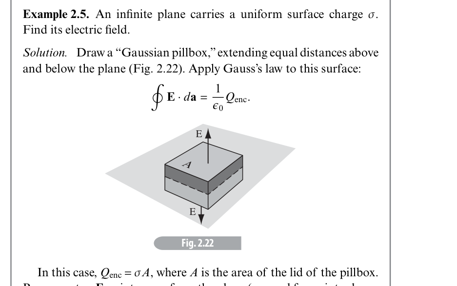
Problem 2.14: Find the electric field a distance $s$ from an infinitely long straight wire that carries a uniform line charge $\lambda$.
習題 2.14:一無限長筆直線載有均勻線電荷密度 $\lambda$。利用高斯定律求距離該線 $s$ 處的電場。
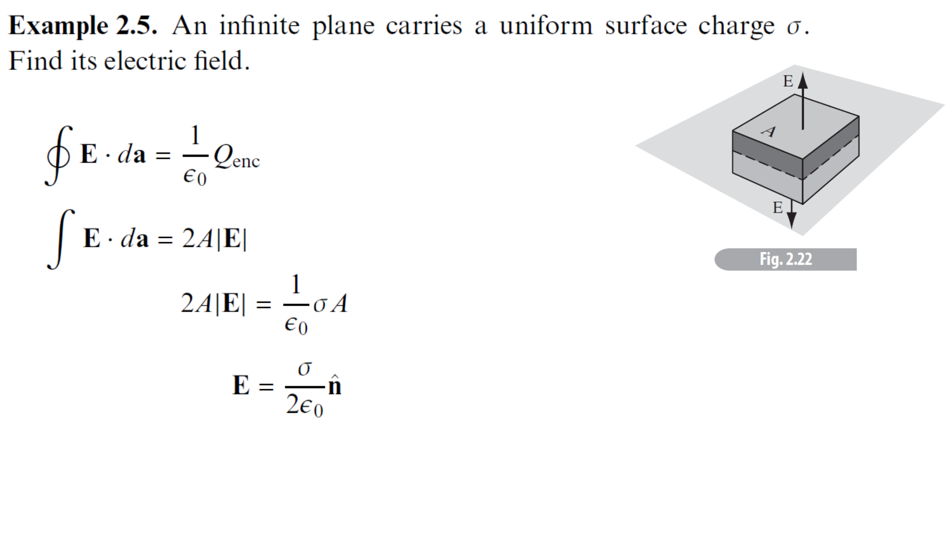
設平面位於 $xy$ 平面。由對稱性可知,電場只能垂直於平面($\pm\hat{\mathbf{z}}$ 方向),向上指向上方,向下指向下方,且大小僅與距離 $|z|$ 相關。
選取跨越帶電平面的「高斯藥丸盒(Pillbox)」,底面積為 $A$:
- 側面通量:法向量平行平面,電場垂直於法向量,側面通量為零。
- 上頂面與下底面:電場與法向量同向,各自貢獻通量 $E A$。
藥丸盒內部包覆之電荷為 $Q_{\text{enc}} = \sigma A$。由高斯定律:
$$2A |E| = \frac{\sigma A}{\epsilon_0} \implies |E| = \frac{\sigma}{2\epsilon_0}$$其中 $\hat{\mathbf{n}}$ 為垂直離開平面的單位法向量。電場與離平面的距離完全無關!
選取半徑為 $s$、長度為 $l$ 的同軸高斯圓柱面。內部包覆電荷為 $Q_{\text{enc}} = \lambda l$。
圓柱側面積為 $2\pi s l$,由柱對稱性:
$$\oint \mathbf{E} \cdot d\mathbf{a} = E(s)(2\pi s l) = \frac{\lambda l}{\epsilon_0}$$此結果與 Example 2.2 之極限 $L\to\infty$ 嚴絲合縫,高斯定律展現了極高的求解效率!
均勻帶電球殼與實心球體之電位分佈求解
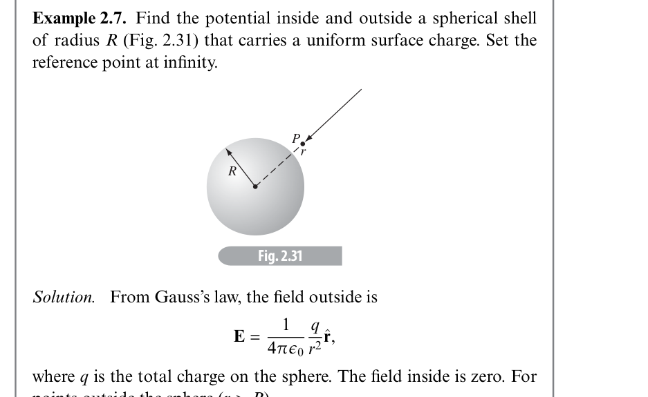
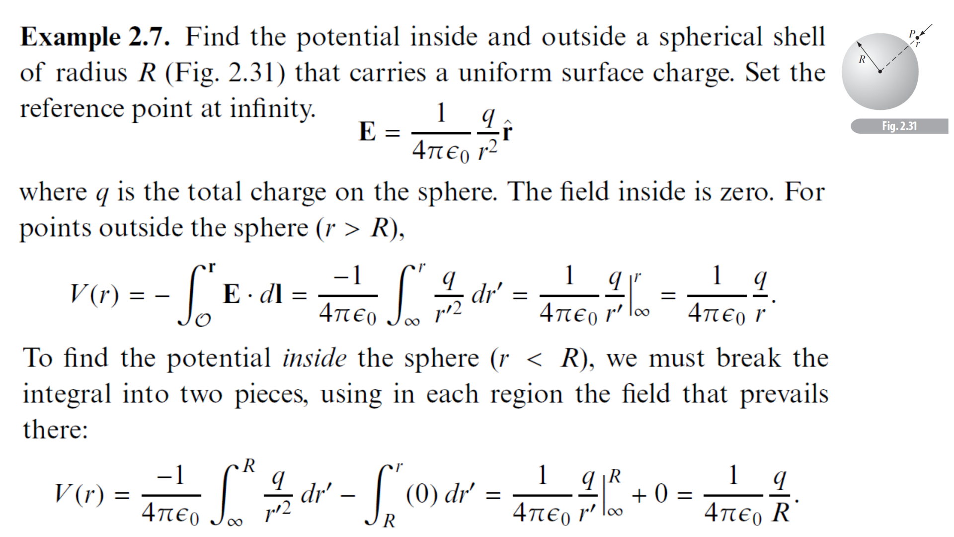
Problem 2.22: Find the potential inside and outside a uniformly charged solid sphere whose radius is $R$ and whose total charge is $q$.
習題 2.22:半徑為 $R$、總電荷為 $q$ 之均勻帶電實心球體,求其內部與外部之電位分佈。
外部電場為 $\mathbf{E} = \frac{1}{4\pi\epsilon_0}\frac{q}{r^2}\hat{\mathbf{r}}$。由電位定義:
$$V(r) = -\int_\infty^r \mathbf{E} \cdot d\mathbf{l} = -\frac{q}{4\pi\epsilon_0} \int_\infty^r \frac{1}{(r')^2} dr' = \left. \frac{q}{4\pi\epsilon_0 r'} \right|_\infty^r$$由於球殼內部無電荷,由高斯定律知內部電場 $\mathbf{E}_{\text{in}} = 0$。求內部電位必須將從 $\infty$ 到 $r$ 的積分路徑分為兩段:
$$V(r) = -\int_\infty^R \mathbf{E}_{\text{out}} \cdot d\mathbf{l} - \int_R^r \mathbf{E}_{\text{in}} \cdot d\mathbf{l} = \left( \frac{1}{4\pi\epsilon_0}\frac{q}{R} \right) - \int_R^r (0)\,dr'$$內部處處為等電位(電位等於表面電位),內部電場 $\mathbf{E} = -\nabla V = 0$ 完全吻合!
外部 ($r \ge R$):與球殼相同,$V(r) = \frac{1}{4\pi\epsilon_0}\frac{q}{r}$。
內部 ($r \le R$):已知內部電場 $\mathbf{E}_{\text{in}} = \frac{1}{4\pi\epsilon_0}\frac{q r}{R^3}\hat{\mathbf{r}}$。分段積分:
$$V(r) = -\int_\infty^R \frac{1}{4\pi\epsilon_0}\frac{q}{(r')^2} dr' - \int_R^r \frac{1}{4\pi\epsilon_0}\frac{q r'}{R^3} dr'$$ $$V(r) = \frac{1}{4\pi\epsilon_0}\frac{q}{R} - \frac{q}{4\pi\epsilon_0 R^3} \left[ \frac{(r')^2}{2} \right]_R^r = \frac{q}{4\pi\epsilon_0 R} - \frac{q}{4\pi\epsilon_0 R^3}\left( \frac{r^2 - R^2}{2} \right)$$球心電位為 $V(0) = \frac{3}{2}\frac{q}{4\pi\epsilon_0 R}$,恰為表面電位的 $1.5$ 倍!
帶電球殼與實心球靜電能量之兩種嚴謹推導方法
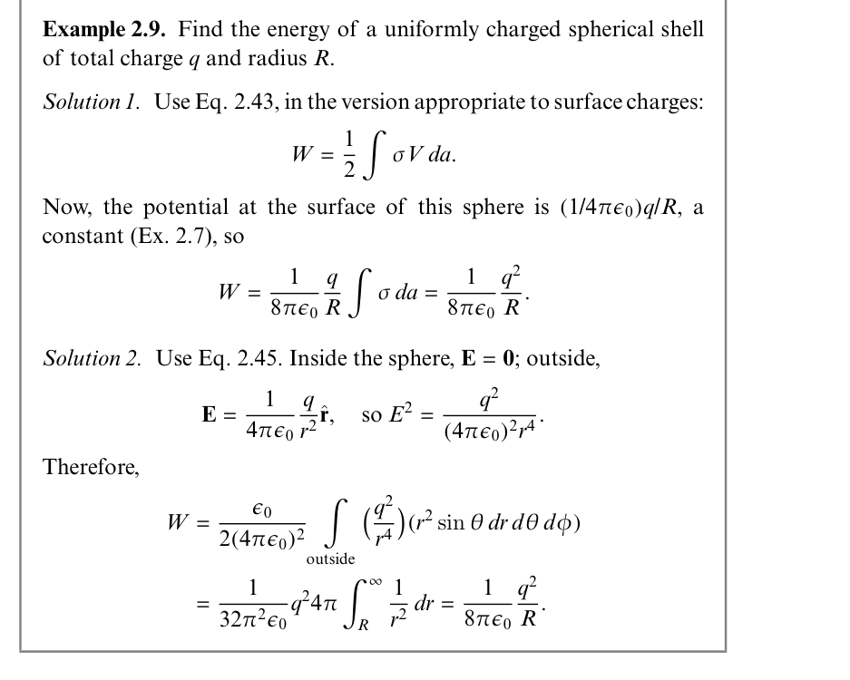
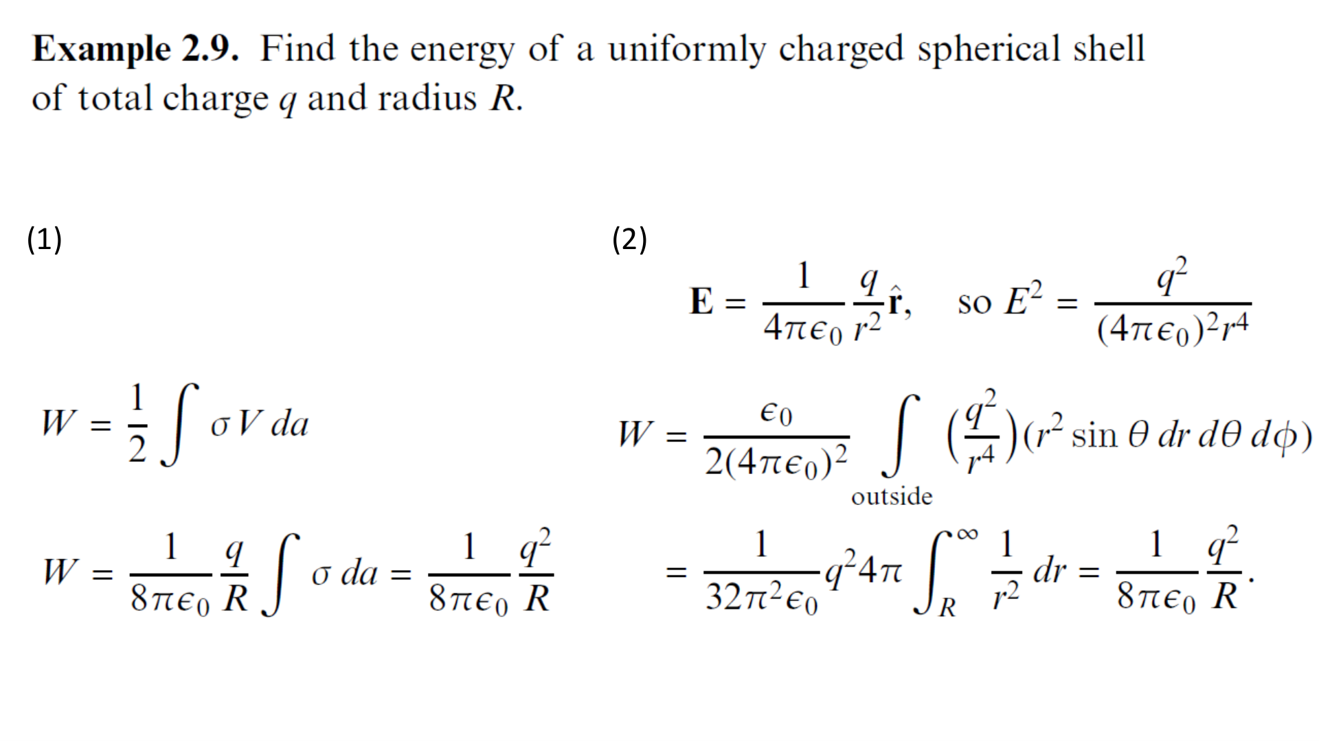
Method (1): $W = \frac{1}{2}\int \sigma V da$
Method (2): $W = \frac{\epsilon_0}{2}\int_{\text{all space}} E^2 d\tau$
Problem 2.35: Find the energy stored in a uniformly charged solid sphere of radius $R$ and total charge $q$.
方法 (1):電荷與電位積分公式 $W = \frac{1}{2}\int \sigma V da$;
方法 (2):電場能量密度體積分公式 $W = \frac{\epsilon_0}{2}\int E^2 d\tau$。
習題 2.35:求均勻帶電實心球體(半徑 $R$、總電荷 $q$)儲存的總靜電能量。
球殼表面電位為常數:$V = \frac{1}{4\pi\epsilon_0}\frac{q}{R}$。
將其提出積分號:
$$W = \frac{1}{2} \int \sigma V da = \frac{1}{2} V \int \sigma da = \frac{1}{2} \left( \frac{1}{4\pi\epsilon_0} \frac{q}{R} \right) q$$電場分佈:內部 $r < R$ 時 $\mathbf{E} = 0$;外部 $r > R$ 時 $\mathbf{E} = \frac{1}{4\pi\epsilon_0}\frac{q}{r^2}\hat{\mathbf{r}}$。
外部電場平方為:$E^2 = \frac{q^2}{(4\pi\epsilon_0)^2 r^4}$。
體積微元為 $d\tau = r^2\sin\theta\,dr\,d\theta\,d\phi = 4\pi r^2 dr$。積分僅需在球殼外($R$ 到 $\infty$)進行:
$$W = \frac{\epsilon_0}{2} \int_{\text{outside}} E^2 d\tau = \frac{\epsilon_0}{2(4\pi\epsilon_0)^2} \int_R^\infty \left( \frac{q^2}{r^4} \right) (4\pi r^2 dr)$$ $$W = \frac{q^2}{32\pi^2 \epsilon_0} (4\pi) \int_R^\infty \frac{1}{r^2} dr = \frac{q^2}{8\pi\epsilon_0} \left[ -\frac{1}{r} \right]_R^\infty = \frac{1}{8\pi\epsilon_0} \frac{q^2}{R}$$兩者結果完全一致!
實心球內部電場 $\mathbf{E}_{\text{in}} = \frac{q r}{4\pi\epsilon_0 R^3}\hat{\mathbf{r}}$,外部電場 $\mathbf{E}_{\text{out}} = \frac{q}{4\pi\epsilon_0 r^2}\hat{\mathbf{r}}$。
將能量分為球內與球外兩部分:
$$W_{\text{in}} = \frac{\epsilon_0}{2} \int_0^R \left( \frac{q r}{4\pi\epsilon_0 R^3} \right)^2 (4\pi r^2 dr) = \frac{q^2}{8\pi\epsilon_0 R^6} \int_0^R r^4 dr = \frac{q^2}{8\pi\epsilon_0 R^6} \frac{R^5}{5} = \frac{1}{40\pi\epsilon_0}\frac{q^2}{R}$$ $$W_{\text{out}} = \frac{\epsilon_0}{2} \int_R^\infty \left( \frac{q}{4\pi\epsilon_0 r^2} \right)^2 (4\pi r^2 dr) = \frac{q^2}{8\pi\epsilon_0} \int_R^\infty \frac{1}{r^2} dr = \frac{1}{8\pi\epsilon_0}\frac{q^2}{R}$$總能量相加:
有限長均勻帶電線段端點上方之電場求解

將線段置於 $x$ 軸上,從 $x = 0$ 延伸到 $x = L$。場點置於原點上方 $(0, 0, z)$。
源點為 $(x, 0, 0)$,分離向量為 $\boldsymbol{r} = -x\hat{\mathbf{x}} + z\hat{\mathbf{z}}$,距離 $r = \sqrt{x^2 + z^2}$。
電場微積分式:
$$\mathbf{E} = \frac{1}{4\pi\epsilon_0} \int_0^L \frac{\lambda dx}{(x^2 + z^2)^{3/2}} (-x\hat{\mathbf{x}} + z\hat{\mathbf{z}})$$水平分量(注意此時由於非對稱,水平分量不為零!):
$$E_x = -\frac{\lambda}{4\pi\epsilon_0} \int_0^L \frac{x dx}{(x^2 + z^2)^{3/2}} = -\frac{\lambda}{4\pi\epsilon_0} \left[ -\frac{1}{\sqrt{x^2 + z^2}} \right]_0^L = \frac{\lambda}{4\pi\epsilon_0} \left[ \frac{1}{\sqrt{L^2 + z^2}} - \frac{1}{z} \right]$$垂直分量:
$$E_z = \frac{\lambda z}{4\pi\epsilon_0} \int_0^L \frac{dx}{(x^2 + z^2)^{3/2}} = \frac{\lambda z}{4\pi\epsilon_0} \left. \frac{x}{z^2 \sqrt{x^2 + z^2}} \right|_0^L = \frac{1}{4\pi\epsilon_0} \frac{\lambda L}{z\sqrt{L^2 + z^2}}$$正方形線圈、均勻帶電圓環與帶電圓盤軸上之電場


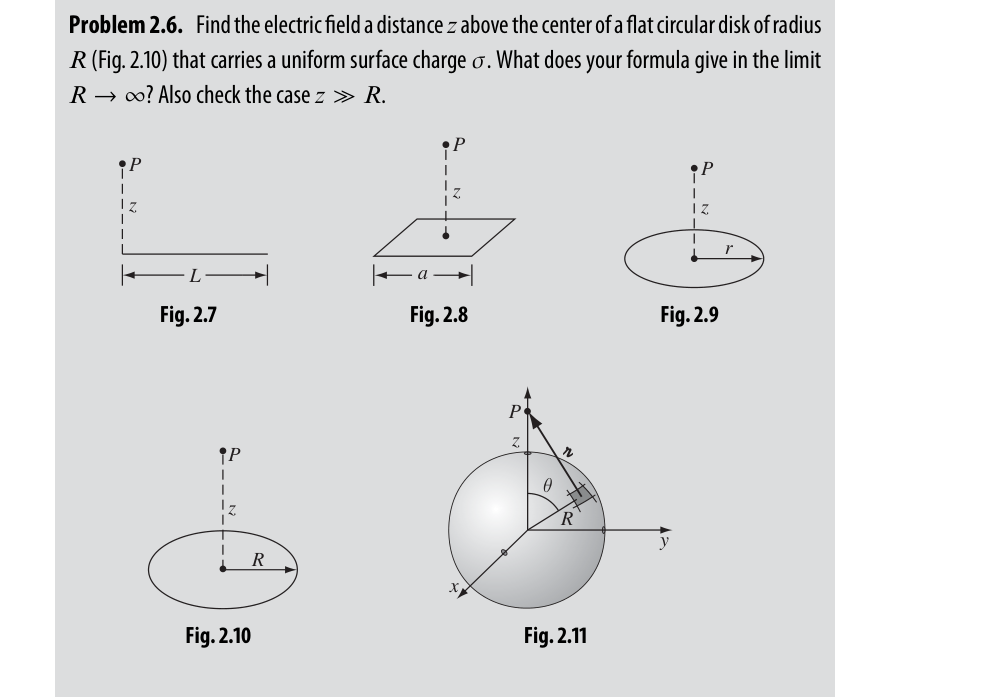
Problem 2.6: Find the electric field a distance $z$ above the center of a flat circular disk of radius $R$ that carries a uniform surface charge $\sigma$. What does your formula give in the limit $R \to \infty$? Also check the case $z \gg R$.
Problem 2.4: Find the electric field a distance $z$ above the center of a square loop (side length $a$) carrying uniform line charge $\lambda$.
習題 2.6:半徑為 $R$ 的均勻帶電圓盤(面電荷密度 $\sigma$),求其中心軸線上距離 $z$ 處的電場。檢驗當 $R \to \infty$ 及 $z \gg R$ 時的極限。
習題 2.4:邊長為 $a$ 的正方形均勻帶電線圈(線電荷密度 $\lambda$),求中心上方 $z$ 處的電場。
由軸對稱性,環上對角微元的水平電場相互抵消,僅存垂直 $z$ 分量:
$$E_z = \oint \frac{1}{4\pi\epsilon_0} \frac{\lambda dl}{r^2 + z^2} \cos\theta = \frac{1}{4\pi\epsilon_0} \frac{\lambda \cos\theta}{r^2 + z^2} \oint dl$$其中 $\cos\theta = \frac{z}{\sqrt{r^2 + z^2}}$,周長 $\oint dl = 2\pi r$:
將圓盤視為許多半徑為 $r$、寬度為 $dr$ 的同心薄圓環之疊加。薄環帶電量為 $dq = \sigma(2\pi r dr)$:
$$E_z = \frac{1}{4\pi\epsilon_0} \int_0^R \frac{(2\pi r dr\,\sigma) z}{(r^2 + z^2)^{3/2}} = \frac{\sigma z}{2\epsilon_0} \int_0^R \frac{r dr}{(r^2 + z^2)^{3/2}}$$定積分計算:$\int_0^R \frac{r dr}{(r^2 + z^2)^{3/2}} = \left[ -\frac{1}{\sqrt{r^2 + z^2}} \right]_0^R = \frac{1}{z} - \frac{1}{\sqrt{R^2 + z^2}}$:
極限 1 ($R \to \infty$):括號內第二項趨於 0,得 $\mathbf{E} \to \frac{\sigma}{2\epsilon_0}\hat{\mathbf{z}}$!精準重現無限大帶電平面高斯解!
極限 2 ($z \gg R$):二項式展開得 $E \approx \frac{\sigma}{2\epsilon_0}\left(1 - (1 - \frac{R^2}{2z^2})\right) = \frac{\sigma \pi R^2}{4\pi\epsilon_0 z^2} = \frac{q_{\text{tot}}}{4\pi\epsilon_0 z^2}$(點電荷極限)。
由 Example 2.2,一條長度為 $2L$ 的線段在垂直距離 $d_{\perp}$ 處產生的垂直電場為 $E = \frac{1}{4\pi\epsilon_0}\frac{2\lambda L}{d_{\perp}\sqrt{d_{\perp}^2 + L^2}}$。
正方形每邊長為 $a$(即 $L = a/2$),邊到中心軸距離為 $a/2$。線段到場點的距離為 $d_{\perp} = \sqrt{z^2 + (a/2)^2}$。
四邊水平分量抵消,垂直分量同向疊加並投影到 $z$ 軸($\cos\phi = z/d_{\perp}$):
立方體頂點電荷通量與無限大帶電平板內部電場
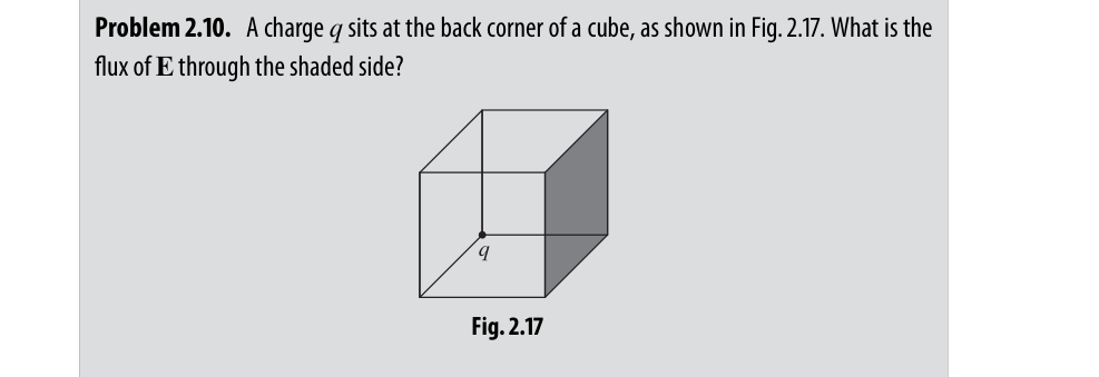

Problem 2.18: An infinite plane slab, of thickness $2d$, carries a uniform volume charge density $\rho$. Find the electric field, as a function of $z$, where $z=0$ is at the center of the slab.
習題 2.18:一無限大厚平板(厚度為 $2d$,範圍 $-d \le z \le d$)具有均勻體電荷密度 $\rho$。以中心面為 $z=0$,求全空間電場 $\mathbf{E}(z)$。
以該頂點為中心,將空間由 8 個相同的立方體共同拼成一個邊長為 $2a$ 的大立方體。點電荷 $q$ 恰好位於大立方體的正中心!
由高斯定律,通過大立方體的總通量為 $\Phi_{\text{total}} = \frac{q}{\epsilon_0}$。由對稱性,通過每一個小立方體的總通量為大立方體的 $1/8$:
$$\Phi_{\text{cube}} = \frac{q}{8\epsilon_0}$$考察該小立方體的 6 個面:
- 與電荷相交的 3 個相鄰面:點電荷發出的電力線完全平行於這 3 個面,電場與面法向量垂直($\mathbf{E} \cdot d\mathbf{a} = 0$),故通量為零!
- 不與電荷相交的 3 個對向面:由對稱性,這 3 個面平分進入該立方體的全部通量:
結論:三個相鄰面通量皆為 0,三個對向面通量皆為 $\frac{q}{24\epsilon_0}$。
由對稱性,在中心面 $z=0$ 處 $\mathbf{E} = 0$。電場沿 $\pm\hat{\mathbf{z}}$ 方向。
選取底面積為 $A$ 的高斯柱,從中心面 $z=0$ 延伸至位置 $z$:
- 板內 ($0 \le z \le d$):包覆電荷 $Q_{\text{enc}} = \rho (A z)$。高斯通量 $\oint \mathbf{E}\cdot d\mathbf{a} = E(z) A$: $$E(z) A = \frac{\rho A z}{\epsilon_0} \implies E(z) = \frac{\rho z}{\epsilon_0}$$
- 板外 ($z \ge d$):包覆電荷已飽和為整個半板厚度 $Q_{\text{enc}} = \rho (A d)$: $$E(z) A = \frac{\rho A d}{\epsilon_0} \implies E(z) = \frac{\rho d}{\epsilon_0} = \frac{\sigma}{2\epsilon_0} \quad (\text{因 } \sigma = 2\rho d)$$
第三章 電位理論、邊界值問題與多極展開 (Potentials)
對應課本 Griffiths Chapter 3 (pp. 113~156)。包含拉普拉斯方程唯一性定理、鏡像電荷法(平面、接地導電球、不接地中性球、帶電球殼)、直角與球座標分離變數法、勒壤得多項式展開、電偶極場與多極展開。
鏡像法經典問題:點電荷與無限大接地導電平面
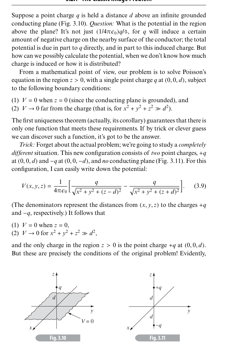
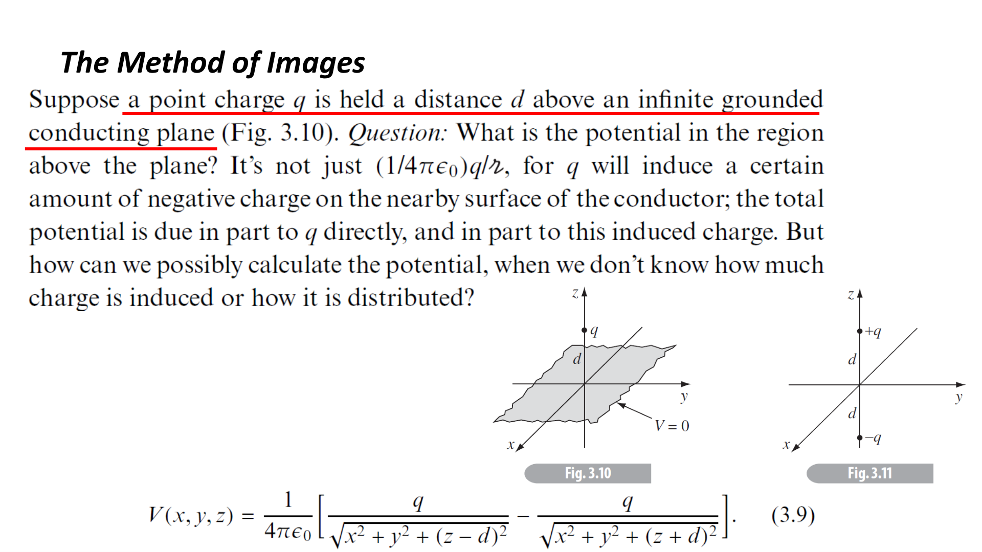
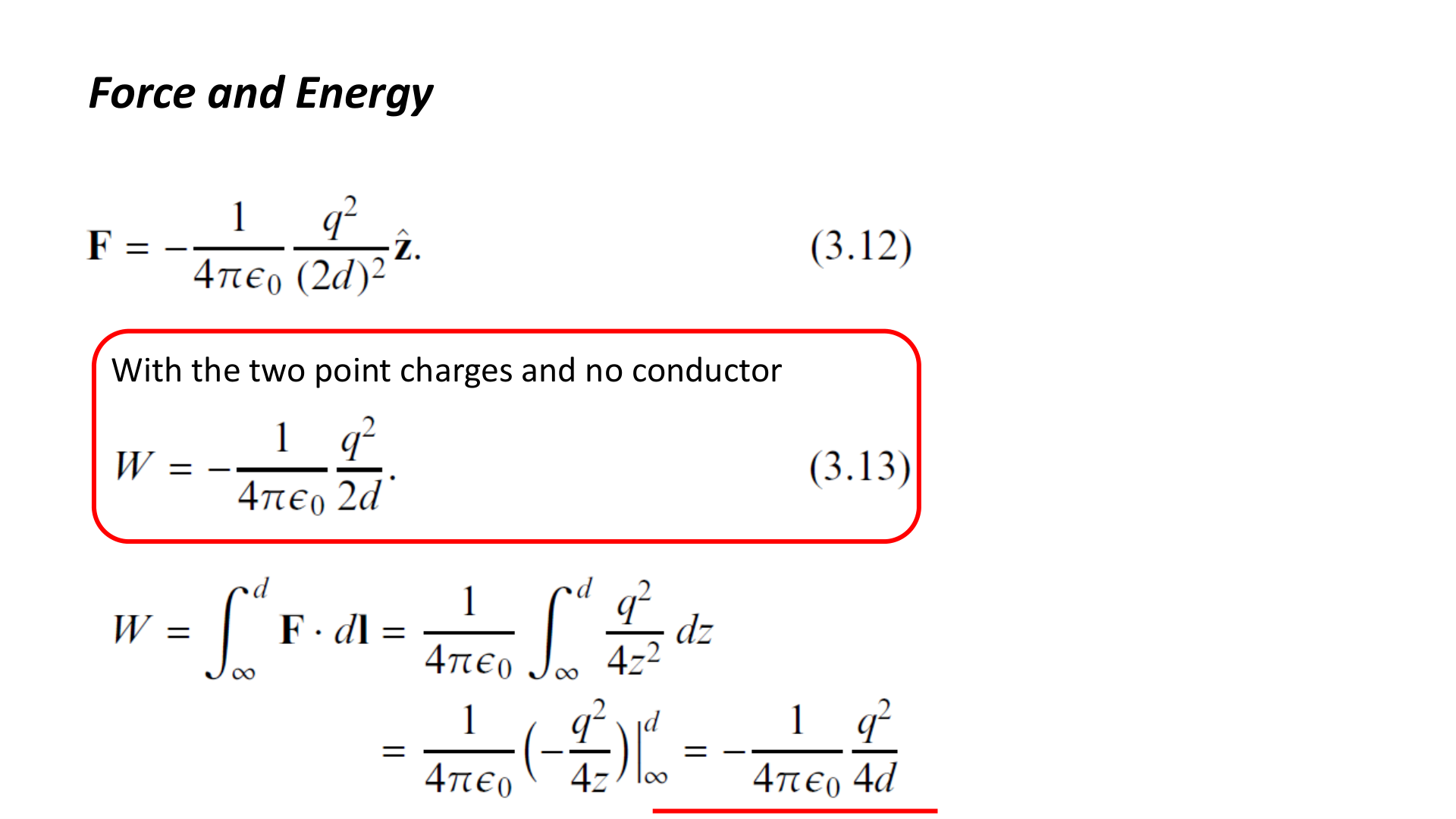
(a) Find the potential $V(x, y, z)$ in the region above the plane ($z > 0$).
(b) Find the induced surface charge density $\sigma(x, y)$ on the plane and the total induced charge $Q$.
(c) Find the force on $q$ and calculate the electrostatic work/energy required to bring $q$ in from infinity.
(a) 求平面上方($z > 0$)區域的電位分佈 $V(x, y, z)$。
(b) 求導電平面上的感應面電荷密度 $\sigma(x, y)$,並積分求全平面之總感應電荷 $Q$。
(c) 求電荷 $q$ 所受之吸力 $\mathbf{F}$,以及將電荷 $q$ 從無窮遠處緩慢移至該處所需作的功(即該系統之靜電能量 $W$)。
- 邊界條件:在區域 $z > 0$ 內,拉普拉斯/帕松方程式為 $\nabla^2 V = -\frac{q}{\epsilon_0}\delta^3(\mathbf{r} - d\hat{\mathbf{z}})$。邊界條件為:(1) 在導電平面上 $V(x, y, 0) = 0$;(2) 在無窮遠處 $V \to 0$。
- 鏡像技巧:在 $z < 0$ 的虛構區域放置鏡像電荷 $-q$ 於 $(0, 0, -d)$,這兩點電荷在 $z=0$ 平面上剛好產生等值反號的電位,精確滿足 $V(z=0)=0$!根據唯一性定理,此電位即為 $z>0$ 區域的唯一真解!
真電荷 $+q$ 位於 $(0, 0, d)$,鏡像電荷 $-q$ 位於 $(0, 0, -d)$。在 $z > 0$ 區域,任意點 $(x, y, z)$ 的電位由兩電荷疊加:
驗證邊界條件:當 $z = 0$ 時,兩分母皆為 $\sqrt{x^2 + y^2 + d^2}$,兩項精確相消,得 $V = 0$;當 $r \to \infty$ 時,$V \to 0$。條件全數滿足!
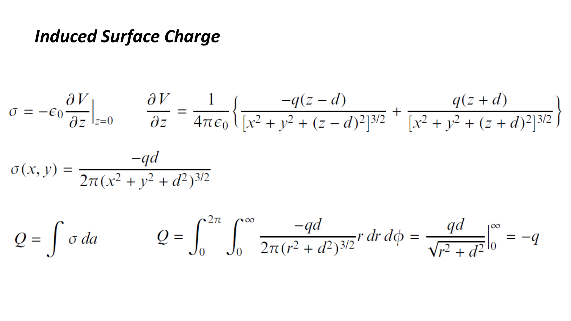
由導體表面邊界條件,感應面電荷密度為:
$$\sigma = -\epsilon_0 \left. \frac{\partial V}{\partial z} \right|_{z=0}$$對 $z$ 求偏微分:
$$\frac{\partial V}{\partial z} = \frac{q}{4\pi\epsilon_0} \left[ \frac{-(z - d)}{\left[ x^2 + y^2 + (z - d)^2 \right]^{3/2}} - \frac{-(z + d)}{\left[ x^2 + y^2 + (z + d)^2 \right]^{3/2}} \right]$$代入 $z = 0$:
$$\left. \frac{\partial V}{\partial z} \right|_{z=0} = \frac{q}{4\pi\epsilon_0} \left[ \frac{d}{(x^2 + y^2 + d^2)^{3/2}} + \frac{d}{(x^2 + y^2 + d^2)^{3/2}} \right] = \frac{1}{4\pi\epsilon_0} \frac{2qd}{(x^2 + y^2 + d^2)^{3/2}}$$因此感應面電荷密度為:
在柱座標下積分全平面求總感應電荷 $Q$(令 $r^2 = x^2 + y^2$,$da = 2\pi r dr$):
$$Q = \int \sigma da = \int_0^\infty \frac{-qd}{2\pi (r^2 + d^2)^{3/2}} (2\pi r dr) = -qd \int_0^\infty \frac{r dr}{(r^2 + d^2)^{3/2}}$$令 $u = r^2 + d^2$,$du = 2r dr$:
$$Q = -qd \left[ -\frac{1}{\sqrt{r^2 + d^2}} \right]_0^\infty = -qd \left( 0 - \left( -\frac{1}{d} \right) \right) = -q$$結論:平面上感應出的總電荷恰為 $-q$!所有由 $+q$ 出發的電力線全數終止於接地平面上!
電荷 $q$ 受到的吸引力即為它與感應電荷(等效於鏡像電荷 $-q$)的作用力。兩者相距 $2d$:
計算將 $q$ 從 $\infty$ 移至 $d$ 所需作的功 $W$:
$$W = -\int_\infty^d \mathbf{F} \cdot d\mathbf{l} = -\int_\infty^d \left( -\frac{1}{4\pi\epsilon_0} \frac{q^2}{4z^2} \right) dz = \frac{q^2}{16\pi\epsilon_0} \left[ -\frac{1}{z} \right]_\infty^d = -\frac{1}{4\pi\epsilon_0} \frac{q^2}{4d}$$接地導電球殼外之點電荷(球對稱鏡像法推導)
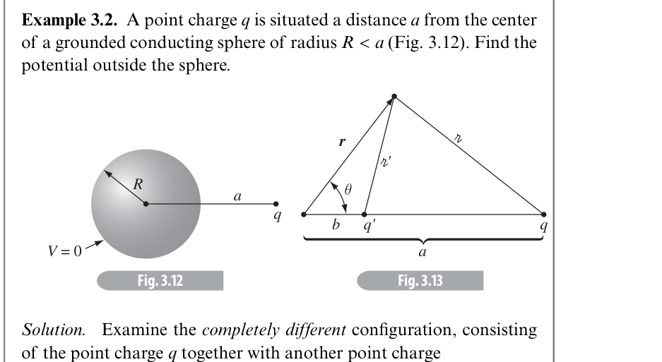
將導電球球心置於原點,電荷 $q$ 位於 $z = d$ 處。球面上電位處處為零:$V(r = a) = 0$。
假設可在球內 $z = b$ 處放置一鏡像電荷 $q'$($b < a$),使得其與 $q$ 在球面上各點產生的電位和為零。
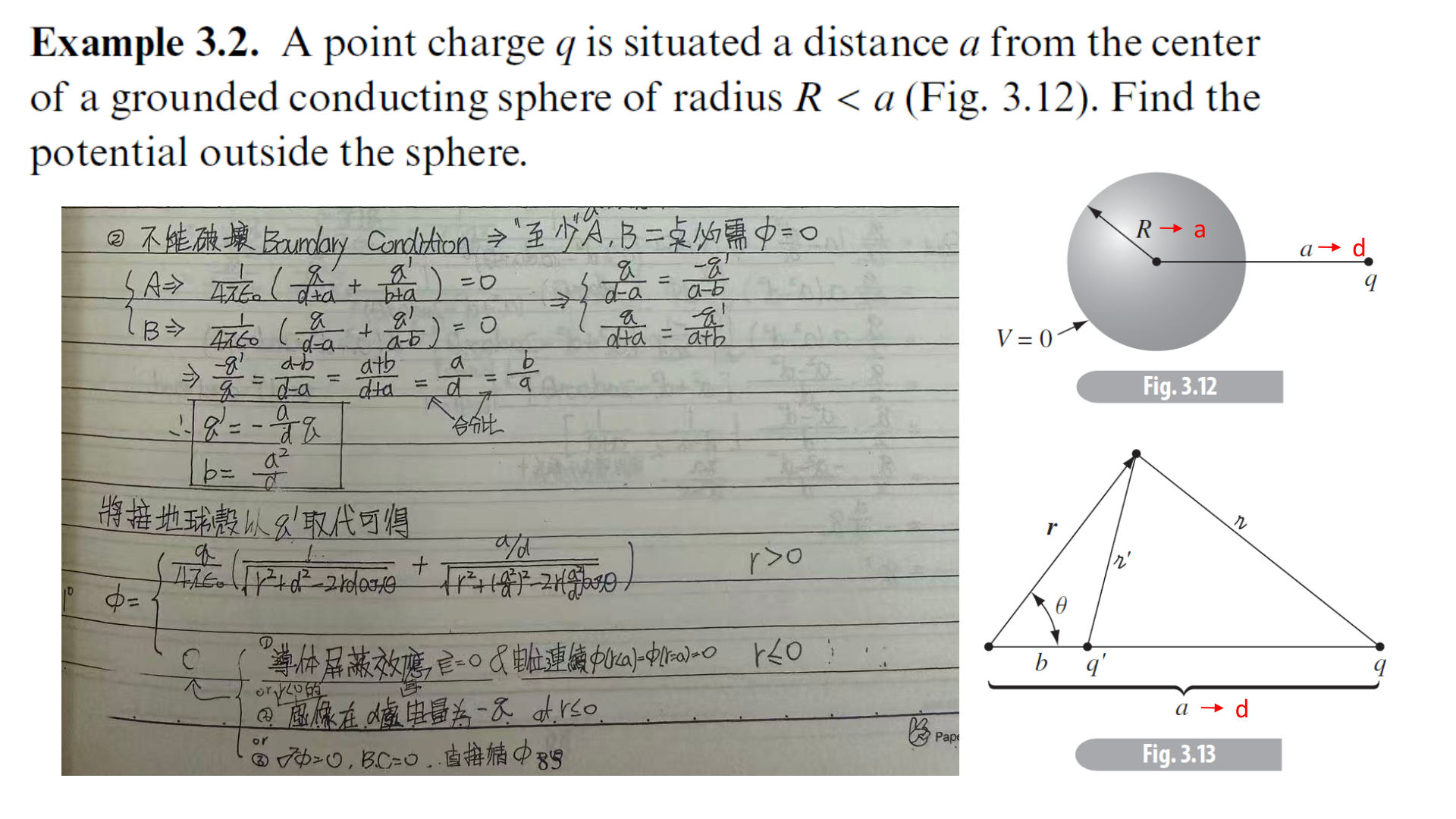
考察球面上與 $z$ 軸相交的兩極點(如講義手稿所示):
- 靠近 $q$ 側之頂點 $A$(坐標 $z = +a$): $$V(A) = \frac{1}{4\pi\epsilon_0} \left( \frac{q}{d - a} + \frac{q'}{a - b} \right) = 0 \implies \frac{q}{d - a} = \frac{-q'}{a - b}$$
- 遠離 $q$ 側之底點 $B$(坐標 $z = -a$): $$V(B) = \frac{1}{4\pi\epsilon_0} \left( \frac{q}{d + a} + \frac{q'}{a + b} \right) = 0 \implies \frac{q}{d + a} = \frac{-q'}{a + b}$$
由兩式相除得:
$$\frac{-q'}{q} = \frac{a - b}{d - a} = \frac{a + b}{d + a}$$根據合分比定理(加比與減比):
$$\frac{(a - b) + (a + b)}{(d - a) + (d + a)} = \frac{2a}{2d} = \frac{a}{d}$$ $$\frac{(a + b) - (a - b)}{(d + a) - (d - a)} = \frac{2b}{2a} = \frac{b}{a}$$因此:
$$\frac{b}{a} = \frac{a}{d} \implies b = \frac{a^2}{d}$$ $$\frac{-q'}{q} = \frac{a}{d} \implies q' = -\frac{a}{d} q$$由餘弦定理,場點 $(r, \theta)$ 到真電荷與鏡像電荷的距離分別為:
$$r_1 = \sqrt{r^2 + d^2 - 2rd\cos\theta}, \quad r_2 = \sqrt{r^2 + b^2 - 2rb\cos\theta} = \sqrt{r^2 + \left(\frac{a^2}{d}\right)^2 - 2r\left(\frac{a^2}{d}\right)\cos\theta}$$故球外電位為:
當 $r = a$ 時,第二項分母提出 $a/d$:
$$\sqrt{a^2 + (a^2/d)^2 - 2a(a^2/d)\cos\theta} = \frac{a}{d}\sqrt{d^2 + a^2 - 2ad\cos\theta}$$與分子 $a/d$ 相消,括號內兩項處處抵消,精確驗證 $V(a, \theta) = 0$!而在導體球內部屏蔽效應,電場 $\mathbf{E}=0$,$V = 0$。
不接地中性導電球殼外之點電荷(雙鏡像電荷疊加)
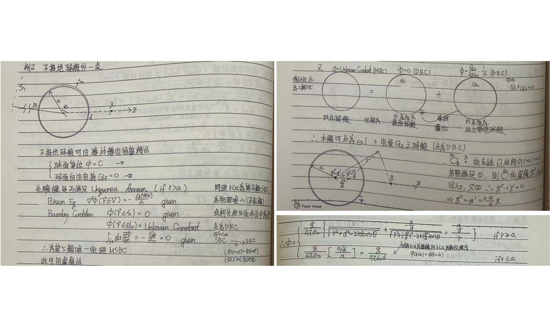
不接地中性球殼的邊界條件為:
- 球體為導體,表面為等電位面:$V(r = a) = V_0 = \text{常數(未知)}$;
- 球體總淨電荷為零:$Q_{\text{net}} = \oint \sigma da = 0$。
如講義 P.10 圖解,可利用線性疊加將本題分解為兩個子系統:
- 系統 1(接地導體球):放置鏡像電荷 $q' = -\frac{a}{d}q$ 於 $b = \frac{a^2}{d}$。此系統使球面上電位 $V = 0$,但球上總感應電荷為 $q' = -\frac{a}{d}q \ne 0$。
- 系統 2(維持中性補償):為滿足球體淨電荷為 0,必須在球內補充電荷 $q'' = -q' = +\frac{a}{d}q$。為了不破壞球面上「等電位」的性質,此補償電荷 $q''$ 必須且只能放置在球心 ($r = 0$)!
置於球心的 $q''$ 在半徑為 $a$ 的球面上產生均勻常數電位 $V_0 = \frac{1}{4\pi\epsilon_0}\frac{q''}{a} = \frac{1}{4\pi\epsilon_0}\frac{q}{d}$!
在球外 ($r \ge a$),電位由真電荷 $q$、鏡像電荷 $q'$ 與球心補償電荷 $q''$ 三者疊加:
在球內及球面上 ($r \le a$),導體為等電位體:
電荷 $q$ 受力為來自 $q'$(吸力,相距 $d - b$)與 $q''$(斥力,相距 $d$)之合力:
$$F = \frac{1}{4\pi\epsilon_0} \left[ \frac{q q'}{(d - b)^2} + \frac{q q''}{d^2} \right] = \frac{q^2}{4\pi\epsilon_0} \left[ -\frac{a/d}{(d - a^2/d)^2} + \frac{a/d}{d^2} \right] = -\frac{q^2 a^3 (2d^2 - a^2)}{4\pi\epsilon_0 d^3 (d^2 - a^2)^2}$$合力始終為吸引力!當 $d \to \infty$ 時,$F \propto -1/d^5$(中性球體受電偶極感應之吸引力)。
帶淨電荷 Q 之導電球殼外之點電荷
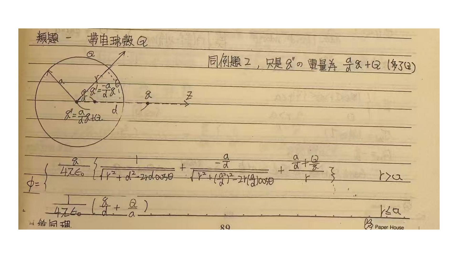
與例題 2 相同,接地所需鏡像電荷為 $q' = -\frac{a}{d}q$(位於 $b = a^2/d$)。
為了使導體球的總淨電荷等於 $Q$,球心補償電荷必須滿足:
$$q_{\text{center}} + q' = Q \implies q'' = Q - q' = Q + \frac{a}{d}q$$將 $q''$ 同樣置於球心,保證球面為等電位面。
球體外部($r \ge a$):
球體內部及表面($r \le a$):
完全精確對應講義 P.11 手寫推導結論!
直角座標分離變數法:二維接地金屬長槽與傅立葉正弦級數
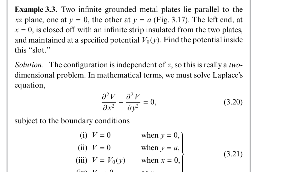
區域內無電荷,電位滿足二維拉普拉斯方程:$\frac{\partial^2 V}{\partial x^2} + \frac{\partial^2 V}{\partial y^2} = 0$。
四個邊界條件(Boundary Conditions):
- (i) $V(x, 0) = 0$(底板接地);
- (ii) $V(x, a) = 0$(頂板接地);
- (iii) $V(0, y) = V_0$(左端給定電位);
- (iv) 當 $x \to \infty$ 時 $V \to 0$(無窮遠處電位歸零)。
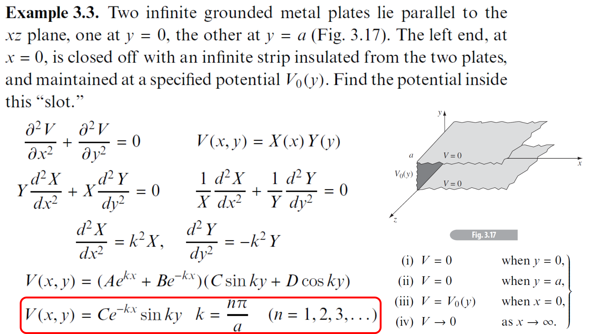
設分離變數解:$V(x, y) = X(x) Y(y)$。代入拉普拉斯方程除以 $XY$:
$$\frac{1}{X}\frac{d^2 X}{dx^2} + \frac{1}{Y}\frac{d^2 Y}{dy^2} = 0 \implies \frac{1}{X}\frac{d^2 X}{dx^2} = k^2, \quad \frac{1}{Y}\frac{d^2 Y}{dy^2} = -k^2$$對於 $X(x)$:通解為 $X(x) = A e^{kx} + B e^{-kx}$。為滿足 (iv) $x\to\infty$ 時 $V\to 0$,必須取 $A = 0$。故 $X(x) = B e^{-kx}$。
對於 $Y(y)$:通解為 $Y(y) = C\sin(ky) + D\cos(ky)$。
- 由 (i) $Y(0) = 0 \implies D = 0$;
- 由 (ii) $Y(a) = 0 \implies \sin(ka) = 0 \implies k a = n\pi \implies k = \frac{n\pi}{a} \quad (n = 1, 2, 3, \dots)$。
故每一本徵模式為:$V_n(x, y) = C_n e^{-n\pi x/a} \sin\left(\frac{n\pi y}{a}\right)$。
由線性疊加原理(Linear combination),一般通解為:
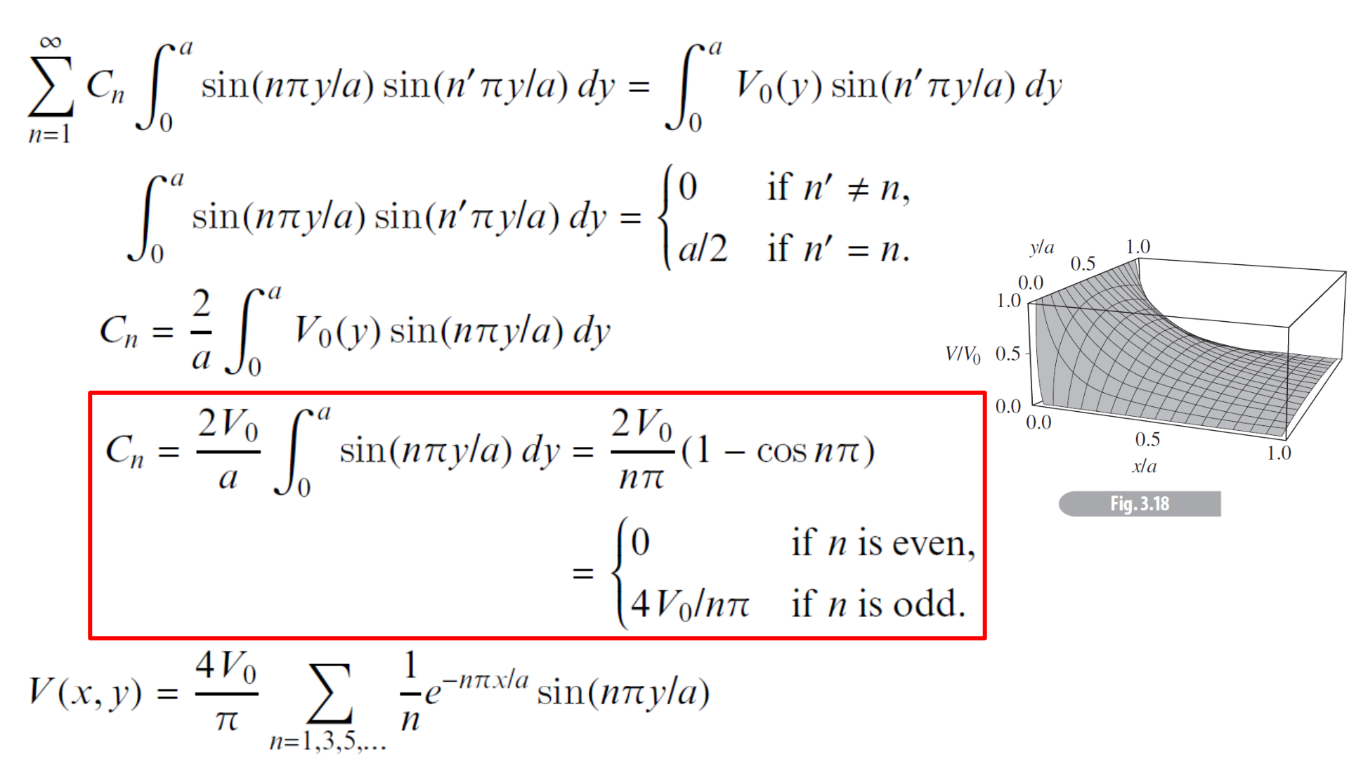
$$V(x, y) = \sum_{n=1}^\infty C_n e^{-n\pi x/a} \sin\left(\frac{n\pi y}{a}\right)$$代入邊界條件 (iii) $x = 0$:
$$V(0, y) = \sum_{n=1}^\infty C_n \sin\left(\frac{n\pi y}{a}\right) = V_0$$利用三角函數正交性(Orthogonality of Sine Functions),兩邊同乘以 $\sin\left(\frac{n'\pi y}{a}\right)$ 並在 $[0, a]$ 上積分:
$$\int_0^a \sin\left(\frac{n\pi y}{a}\right) \sin\left(\frac{n'\pi y}{a}\right) dy = \frac{a}{2} \delta_{n n'}$$ $$C_n \left(\frac{a}{2}\right) = \int_0^a V_0 \sin\left(\frac{n\pi y}{a}\right) dy = V_0 \left[ -\frac{a}{n\pi} \cos\left(\frac{n\pi y}{a}\right) \right]_0^a = \frac{a V_0}{n\pi} (1 - \cos n\pi)$$由於 $1 - \cos n\pi = \begin{cases} 0 & n \text{ 為偶數} \\ 2 & n \text{ 為奇數} \end{cases}$,解得:
最終電位級數解為:
矩形金屬導電管之雙曲函數與三維分離變數邊界值問題
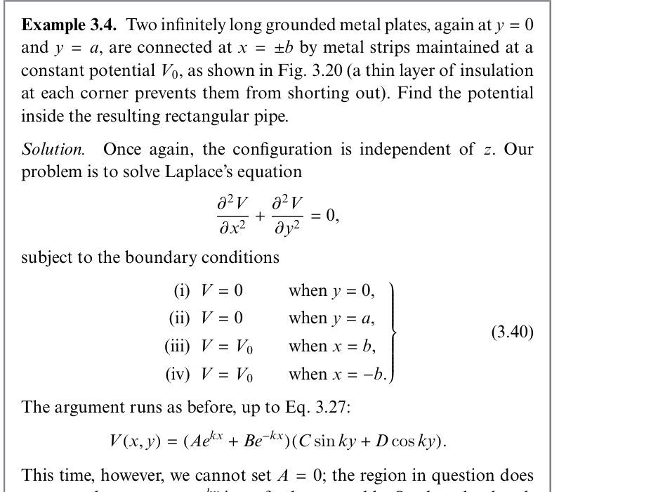
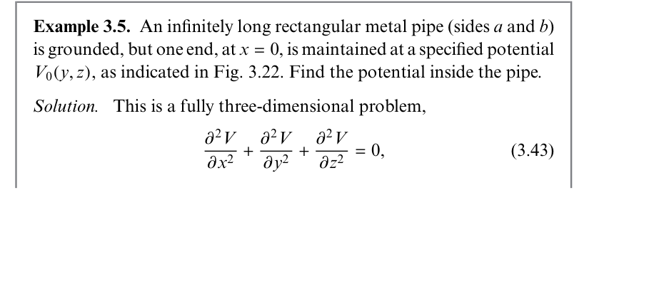
Example 3.5: An infinitely long rectangular metal pipe (sides $a$ and $b$) is grounded, but one end, at $x = 0$, is maintained at a specified potential $V_0(y, z)$ (Fig. 3.22). Find the potential inside the pipe.
例題 3.5:一無限長三維矩形導電管,四個側面($y=0, a$ 及 $z=0, b$)全部接地,底端 $x=0$ 處維持給定電位 $V_0(y, z)$。求管內的電位分佈 $V(x, y, z)$。
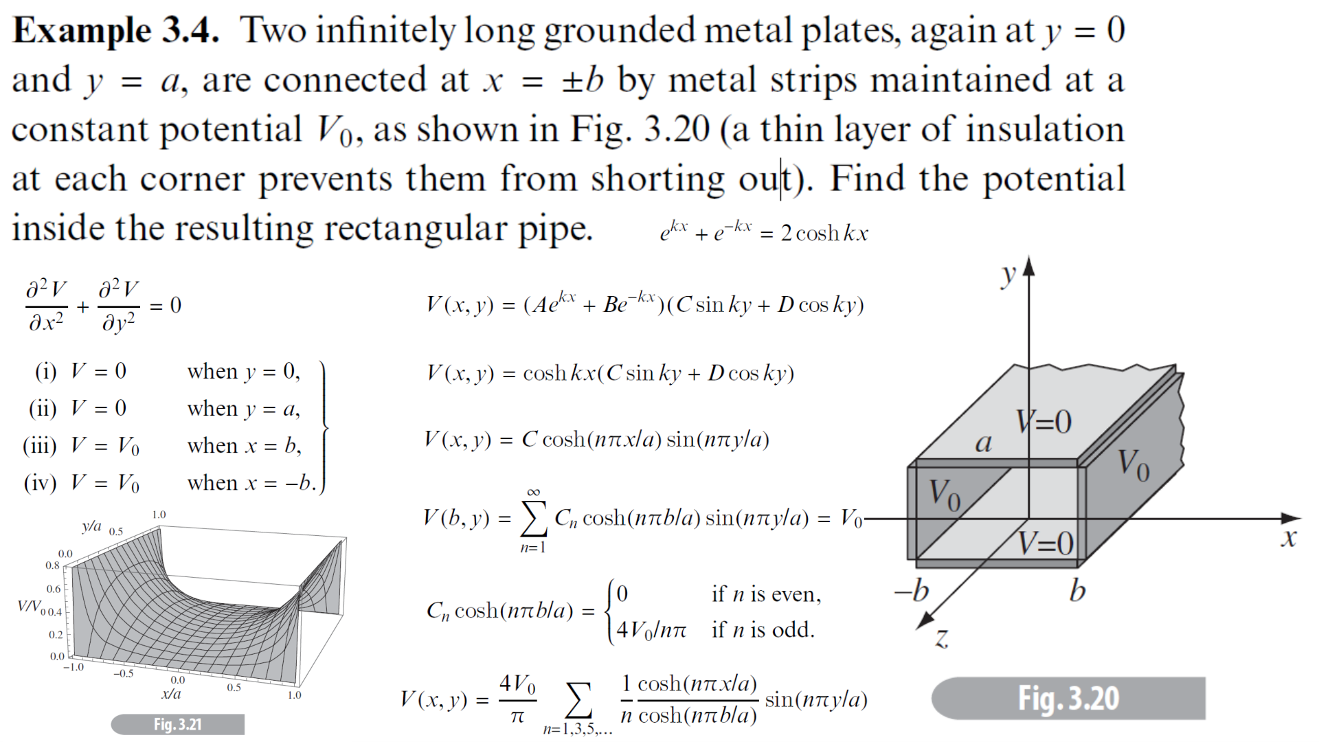
因兩側邊界 $x = \pm b$ 皆為 $V_0$,系統關於 $x = 0$ 具有偶對稱性(Even Symmetry):$V(-x, y) = V(x, y)$。
在 $X(x) = A e^{kx} + B e^{-kx}$ 中,偶函數組合為雙曲餘弦:
$$X(x) = \cosh(kx) = \frac{e^{kx} + e^{-kx}}{2}$$對於 $y$ 方向,邊界 $y=0$ 與 $y=a$ 接地,依然為 $Y(y) = \sin(n\pi y/a)$,$k = n\pi/a$。疊加得:
$$V(x, y) = \sum_{n=1}^\infty C_n \cosh\left(\frac{n\pi x}{a}\right) \sin\left(\frac{n\pi y}{a}\right)$$在邊界 $x = b$ 處,代入 $V(b, y) = V_0$:
$$\sum_{n=1}^\infty \left[ C_n \cosh\left(\frac{n\pi b}{a}\right) \right] \sin\left(\frac{n\pi y}{a}\right) = V_0$$此與 Ex 3.3 完全等價,故有效係數為:
$$C_n \cosh\left(\frac{n\pi b}{a}\right) = \begin{cases} 0 & n \text{ 為偶數} \\ \frac{4V_0}{n\pi} & n \text{ 為奇數} \end{cases}$$設 $V(x, y, z) = X(x) Y(y) Z(z)$。三維拉普拉斯方程分離為:
$$\frac{1}{X}\frac{d^2 X}{dx^2} = k^2 + l^2, \quad \frac{1}{Y}\frac{d^2 Y}{dy^2} = -k^2, \quad \frac{1}{Z}\frac{d^2 Z}{dz^2} = -l^2$$由 $Y(0)=Y(a)=0 \implies k = \frac{n\pi}{a}$,$Y(y) = \sin(n\pi y/a)$;
由 $Z(0)=Z(b)=0 \implies l = \frac{m\pi}{b}$,$Z(z) = \sin(m\pi z/b)$;
當 $x \to \infty$ 時 $V \to 0$,故 $X(x) = e^{-\gamma_{n,m} x}$,其中衰減常數為 $\gamma_{n,m} = \pi\sqrt{(n/a)^2 + (m/b)^2}$。
通解為雙重傅立葉級數:
由雙重正交性,展開係數為:$C_{n,m} = \frac{4}{ab}\int_0^a \int_0^b V_0(y, z)\sin(n\pi y/a)\sin(m\pi z/b)\,dy\,dz$。
球座標分離變數法:勒壤得多項式展開與均勻外電場導電球
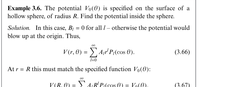
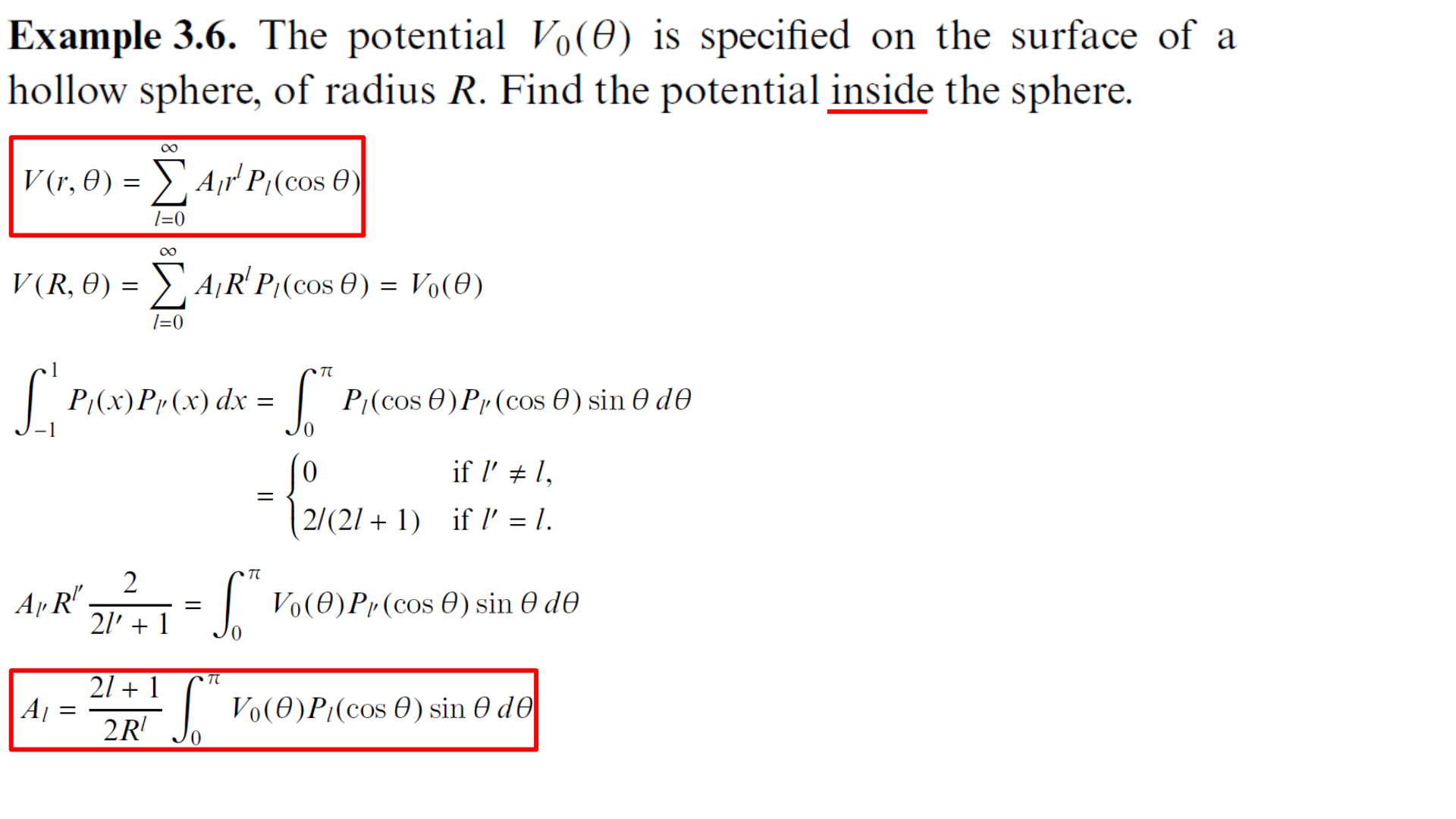
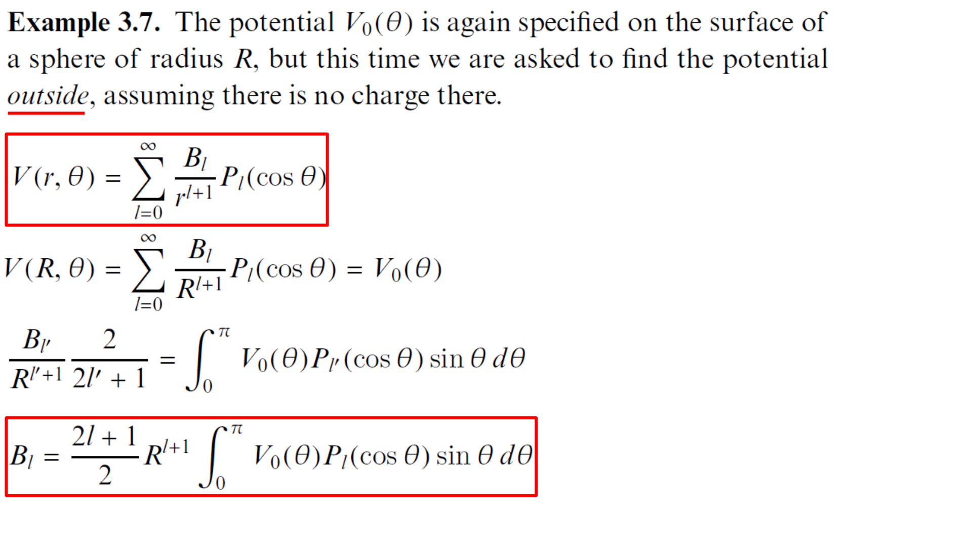
Example 3.7: The potential $V_0(\theta)$ is again specified on the surface of a sphere of radius $R$, but this time we are asked to find the potential outside, assuming there is no charge there.
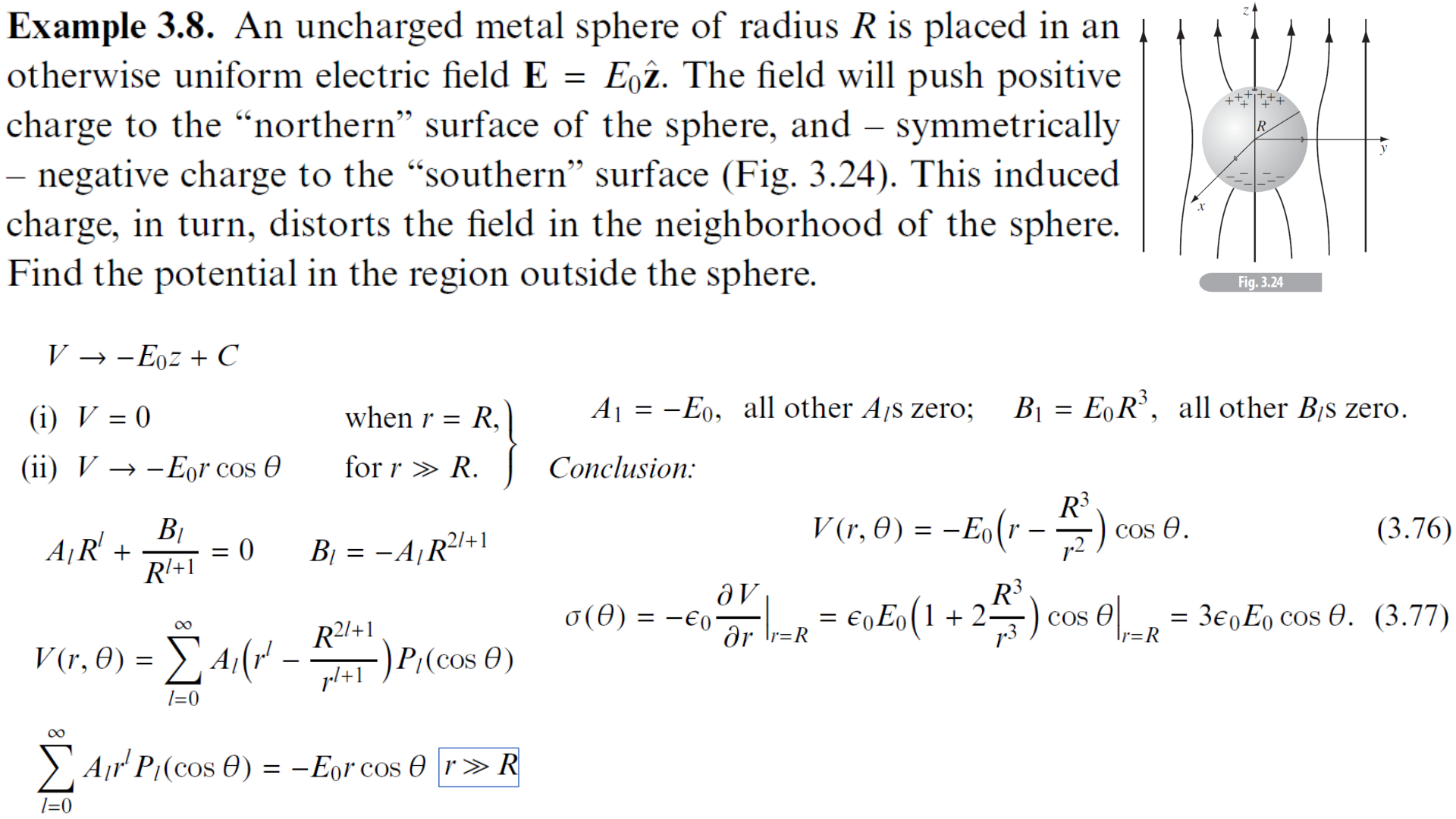
Example 3.8: An uncharged metal sphere of radius $R$ is placed in an otherwise uniform electric field $\mathbf{E} = E_0\hat{\mathbf{z}}$. Find the potential in the region outside the sphere, and the induced surface charge density $\sigma(\theta)$.
例題 3.7:半徑為 $R$ 的球面給定電位分佈 $V_0(\theta)$。求球體外部(無電荷區域)的電位 $V(r, \theta)$。
例題 3.8:一不帶電之金屬球(半徑 $R$)置入原本均勻的外加電場 $\mathbf{E} = E_0\hat{\mathbf{z}}$ 中。求球外的電位分佈以及金屬球表面的感應面電荷密度 $\sigma(\theta)$。
具軸對稱性(無 $\phi$ 依賴)時,拉普拉斯方程的分離變數通解為:
$$V(r, \theta) = \sum_{l=0}^\infty \left( A_l r^l + \frac{B_l}{r^{l+1}} \right) P_l(\cos\theta)$$其中 $P_l(x)$ 為第 $l$ 階勒壤得多項式(Legendre Polynomials),滿足正交性:
$$\int_0^\pi P_l(\cos\theta) P_{l'}(\cos\theta) \sin\theta\,d\theta = \frac{2}{2l + 1} \delta_{l l'}$$在球心 $r = 0$ 處,電位必須為有限值,不能發散。因此所有 $B_l$ 必須全為零($B_l = 0$):
$$V(r, \theta) = \sum_{l=0}^\infty A_l r^l P_l(\cos\theta)$$在球表面 $r = R$ 處匹配邊界條件 $V(R, \theta) = V_0(\theta)$:
$$\sum_{l=0}^\infty A_l R^l P_l(\cos\theta) = V_0(\theta)$$利用勒壤得多項式之正交性,兩邊同乘 $P_{l'}(\cos\theta)\sin\theta$ 積分得:
在無窮遠處 $r \to \infty$,電位趨近於 0,不能發散。因此所有 $A_l$ 必須為零($A_l = 0$):
$$V(r, \theta) = \sum_{l=0}^\infty \frac{B_l}{r^{l+1}} P_l(\cos\theta)$$同理在表面匹配正交性,解得:
邊界條件:
- (i) 金屬球表面等電位,取其電位為零:$V(R, \theta) = 0$;
- (ii) 當 $r \gg R$ 時,恢復均勻電場 $\mathbf{E}_0 = E_0\hat{\mathbf{z}} \implies V \to -E_0 z = -E_0 r\cos\theta$。
由邊界條件 (ii),當 $r \to \infty$ 時:
$$\sum_{l=0}^\infty A_l r^l P_l(\cos\theta) \to -E_0 r P_1(\cos\theta) \quad (\text{因 } P_1(\cos\theta) = \cos\theta)$$直接比對各階係數:只有 $l = 1$ 的項存在,且:
$$A_1 = -E_0, \quad A_l = 0 \; (\forall l \ne 1)$$再由邊界條件 (i) $V(R, \theta) = 0$:
$$\left( A_l R^l + \frac{B_l}{R^{l+1}} \right) = 0 \implies B_l = -A_l R^{2l+1}$$當 $l \ne 1$ 時,$A_l = 0 \implies B_l = 0$;當 $l = 1$ 時:
$$B_1 = -(-E_0) R^{2(1)+1} = E_0 R^3$$將 $A_1$ 與 $B_1$ 代回通解,即得著名的外部電位公式:
物理意義:第一項 $-E_0 r\cos\theta$ 是外加背景均勻電場的電位;第二項 $\frac{E_0 R^3\cos\theta}{r^2}$ 恰為一個位於球心、電偶極矩大小為 $p = 4\pi\epsilon_0 R^3 E_0$ 的感應電偶極(Induced Dipole)所建立的電場!
計算感應面電荷密度 $\sigma(\theta)$:
$$\sigma(\theta) = -\epsilon_0 \left. \frac{\partial V}{\partial r} \right|_{r=R} = -\epsilon_0 \left. \left[ -E_0 \left( 1 + \frac{2R^3}{r^3} \right) \cos\theta \right] \right|_{r=R} = \epsilon_0 E_0 (1 + 2)\cos\theta$$北半球($\cos\theta > 0$)感應正電荷,南半球($\cos\theta < 0$)感應負電荷,赤道處為 0,整體呈完美的電偶極電荷分佈!
物理電偶極遠距電位(多極展開)與電偶極電場公式
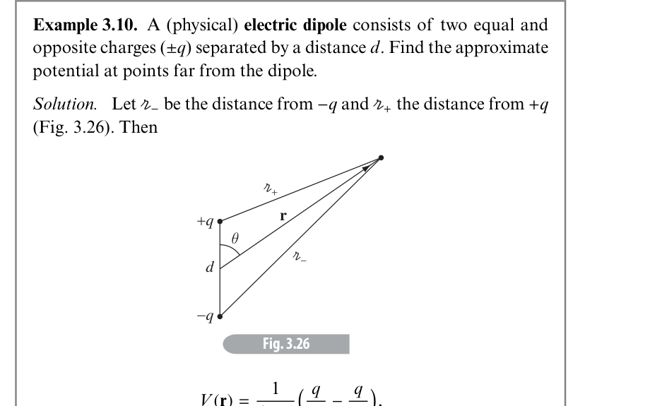
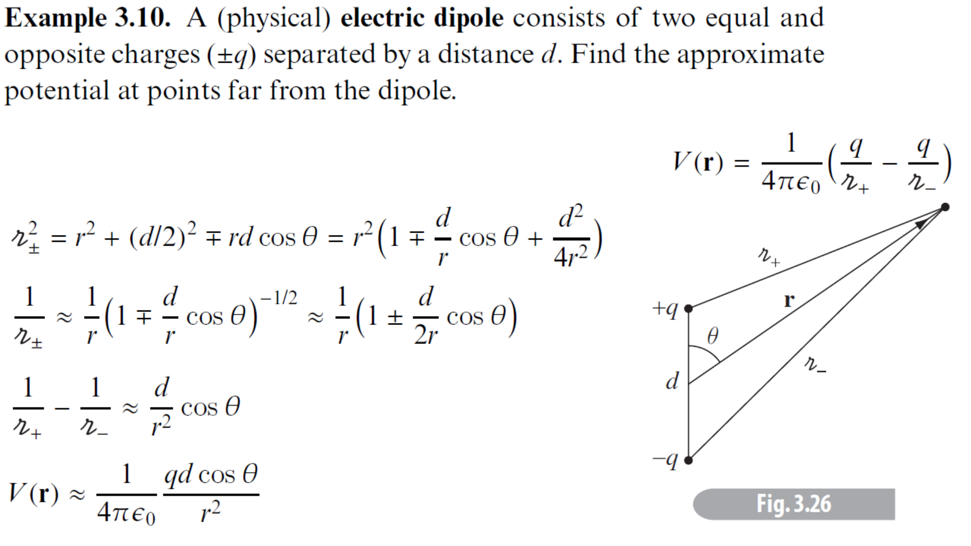
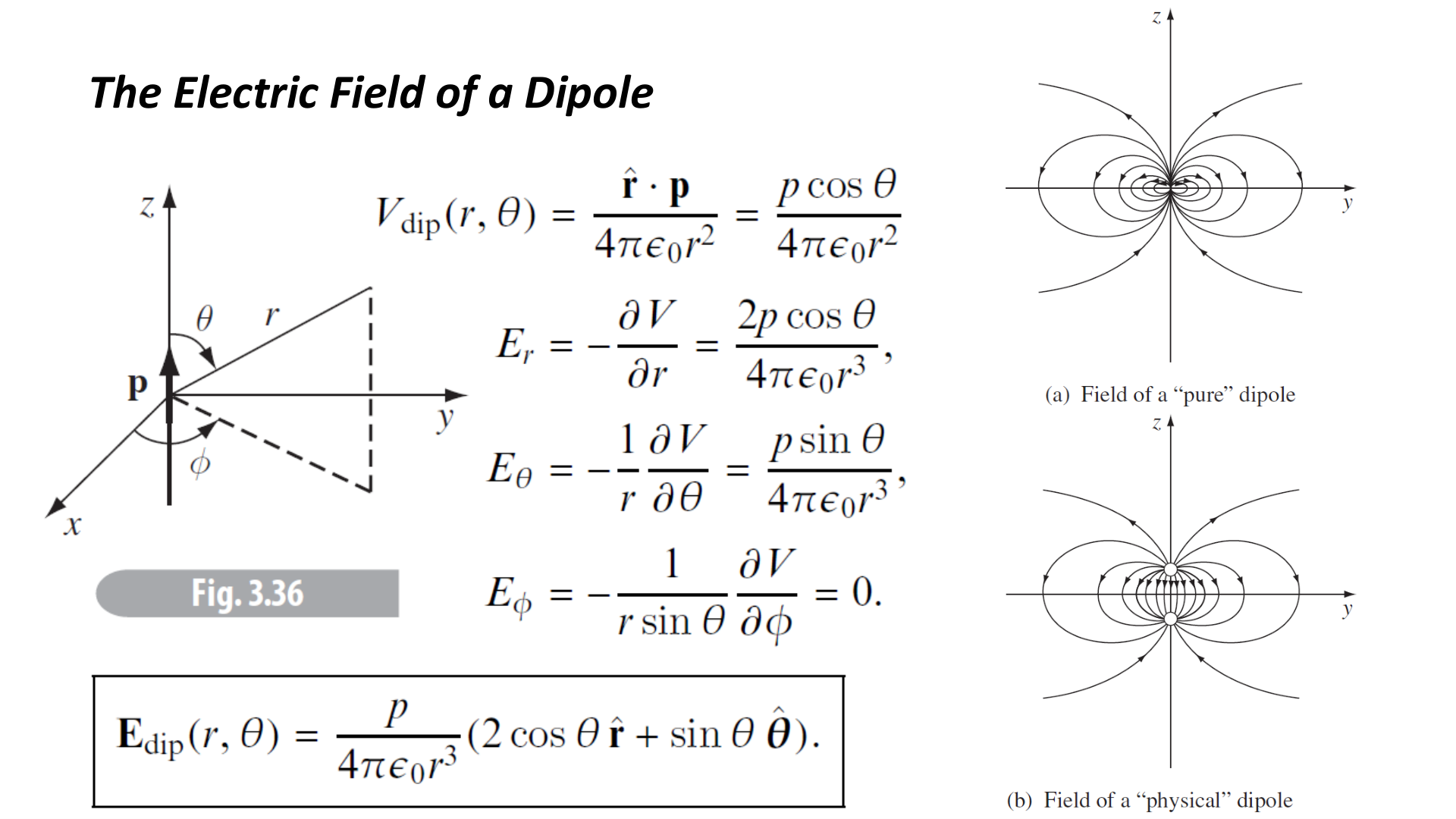
Section 3.4.4 / Lecture P.25: Determine the electric field of an ideal electric dipole by taking the negative gradient of the dipole potential.
講義 P.25 重點:對此電位取負梯度 $-\nabla V$,推導出理想點電偶極的電場分佈公式 $\mathbf{E}_{\text{dip}}(r, \theta)$。
設正電荷 $+q$ 位於 $(0, 0, d/2)$,負電荷 $-q$ 位於 $(0, 0, -d/2)$。場點為 $(r, \theta)$。
到正負電荷的距離平方為:
$$r_\pm^2 = r^2 + (d/2)^2 \mp r d\cos\theta = r^2 \left( 1 \mp \frac{d}{r}\cos\theta + \frac{d^2}{4r^2} \right)$$取倒數並進行一階泰勒/二項式展開($(1 + x)^{-1/2} \approx 1 - \frac{1}{2}x$):
$$\frac{1}{r_\pm} \approx \frac{1}{r} \left( 1 \mp \frac{d}{r}\cos\theta \right)^{-1/2} \approx \frac{1}{r} \left( 1 \pm \frac{d}{2r}\cos\theta \right)$$兩者相減:
$$\frac{1}{r_+} - \frac{1}{r_-} \approx \frac{1}{r} \left( 1 + \frac{d}{2r}\cos\theta \right) - \frac{1}{r} \left( 1 - \frac{d}{2r}\cos\theta \right) = \frac{d\cos\theta}{r^2}$$電位疊加為:
$$V(\mathbf{r}) = \frac{q}{4\pi\epsilon_0} \left( \frac{1}{r_+} - \frac{1}{r_-} \right) \approx \frac{1}{4\pi\epsilon_0} \frac{qd\cos\theta}{r^2}$$定義物理電偶極矩向量為 $\mathbf{p} = q\mathbf{d} = qd\,\hat{\mathbf{z}}$。由於 $\mathbf{p} \cdot \hat{\mathbf{r}} = p\cos\theta$:
在球座標系中,梯度算子為:$\nabla V = \frac{\partial V}{\partial r}\hat{\mathbf{r}} + \frac{1}{r}\frac{\partial V}{\partial \theta}\hat{\boldsymbol{\theta}} + \frac{1}{r\sin\theta}\frac{\partial V}{\partial \phi}\hat{\boldsymbol{\phi}}$。
對電偶極電位取負梯度 $\mathbf{E} = -\nabla V$:
- 徑向分量: $$E_r = -\frac{\partial V}{\partial r} = -\frac{\partial}{\partial r}\left( \frac{p\cos\theta}{4\pi\epsilon_0 r^2} \right) = \frac{2p\cos\theta}{4\pi\epsilon_0 r^3}$$
- 天頂角分量: $$E_\theta = -\frac{1}{r}\frac{\partial V}{\partial \theta} = -\frac{1}{r}\left( \frac{-p\sin\theta}{4\pi\epsilon_0 r^2} \right) = \frac{p\sin\theta}{4\pi\epsilon_0 r^3}$$
- 方位角分量:由軸對稱性 $E_\phi = 0$。
綜合寫為向量形式:
無座標的純向量形式(課本 Eq. 3.104):
拉普拉斯方程性質、平均值定理與恩紹定理 (Earnshaw's Theorem)
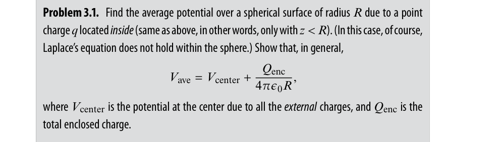
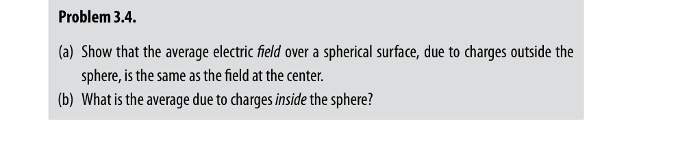
Problem 3.4 (Earnshaw's Theorem): Prove that a charged particle cannot be held in a stable equilibrium position by electrostatic forces alone.
習題 3.4(恩紹定理 Earnshaw's Theorem):試證明:單靠靜電力,帶電粒子絕不可能在自由空間中處於穩定的力學平衡位置。
一維拉普拉斯方程為 $\frac{d^2 V}{dx^2} = 0$。直接兩次積分:
$$V(x) = m x + b$$其中 $m, b$ 為常數。其二階導數處處為零,故不存在曲率改變,無任何局部極大值或極小值(一條斜直線的極值必在區間兩端點)。
同時,在任意點 $x$ 兩側對稱距離 $a$ 的平均值為:
$$\frac{V(x + a) + V(x - a)}{2} = \frac{[m(x+a)+b] + [m(x-a)+b]}{2} = mx + b = V(x)$$證明了一維的平均值定理!
設正電荷 $q$ 位於空間中某平衡點 $P$。若該點為穩定平衡點(Stable Equilibrium),則粒子無論沿任何方向發生微小位移,都必須受到指向平衡點的恢復力(Restoring Force):
$$\mathbf{F} = q\mathbf{E} \implies \mathbf{E} \text{ 必須從各方向皆指向 } P$$以 $P$ 為中心取一任意小的球面高斯面 $S$。由於電場 $\mathbf{E}$ 在整個球面上處處指向球心 $P$,電場的向外總通量必為負值:
$$\oint_S \mathbf{E} \cdot d\mathbf{a} < 0$$然而根據高斯定律,$\oint_S \mathbf{E}\cdot d\mathbf{a} = \frac{Q_{\text{enc}}}{\epsilon_0}$。在無外部電荷存在的自由空間中,內部並無其他固定電荷產生源,故必有:
$$\oint_S \mathbf{E} \cdot d\mathbf{a} = 0$$產生矛盾!因此電場不可能在所有方向上都指向 $P$。以電位觀點而言,穩定平衡要求電位具有局部極小值($\nabla^2 V > 0$),但拉普拉斯方程要求 $\nabla^2 V = 0$(鞍點 Saddle Point),故穩定平衡在純靜電場中不可能實現!
無限長帶電直線與接地導電平面的鏡像解與感應面電荷
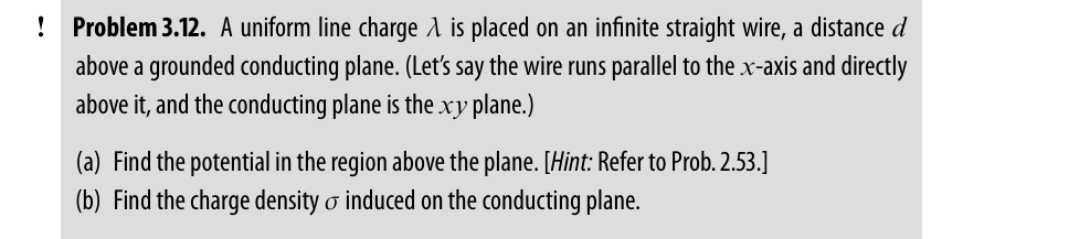
(a) Find the potential in the region above the plane ($z > 0$).
(b) Find the charge density $\sigma$ induced on the conducting plane.
(a) 求平面上方($z > 0$)區域的電位分佈 $V(y, z)$。
(b) 求接地導電平面上的感應面電荷密度 $\sigma(y)$。
在 $z = -d$ 處放置一條平行的鏡像直線,帶電量為 $-\lambda$。
單一長直線距離 $s$ 處的電位為 $V = -\frac{\lambda}{2\pi\epsilon_0}\ln(s)$。兩導線疊加:
$$V(y, z) = -\frac{\lambda}{2\pi\epsilon_0} \ln(s_+) + \frac{\lambda}{2\pi\epsilon_0} \ln(s_-) = \frac{\lambda}{2\pi\epsilon_0} \ln\left( \frac{s_-}{s_+} \right)$$其中 $s_+ = \sqrt{y^2 + (z - d)^2}$,$s_- = \sqrt{y^2 + (z + d)^2}$:
驗證:在 $z = 0$ 處,$s_- = s_+$,對數項為 $\ln(1) = 0 \implies V(y, 0) = 0$!完全滿足接地條件。
利用導體表面邊界條件:$\sigma(y) = -\epsilon_0 \left. \frac{\partial V}{\partial z} \right|_{z=0}$:
$$\frac{\partial V}{\partial z} = \frac{\lambda}{4\pi\epsilon_0} \left[ \frac{2(z + d)}{y^2 + (z + d)^2} - \frac{2(z - d)}{y^2 + (z - d)^2} \right]$$在 $z = 0$ 處代入:
$$\left. \frac{\partial V}{\partial z} \right|_{z=0} = \frac{\lambda}{4\pi\epsilon_0} \left[ \frac{2d}{y^2 + d^2} - \frac{-2d}{y^2 + d^2} \right] = \frac{\lambda}{\pi\epsilon_0} \frac{d}{y^2 + d^2}$$驗證單位長度總感應電荷:$\int_{-\infty}^\infty \sigma(y) dy = -\frac{\lambda d}{\pi} \left. \frac{1}{d}\arctan(y/d) \right|_{-\infty}^\infty = -\lambda$,完全等於 $-\lambda$!
球殼邊界電荷 $\sigma(\theta) = k\cos\theta$ 與邊界電位 $V_0\cos(3\theta)$ 之分離變數解
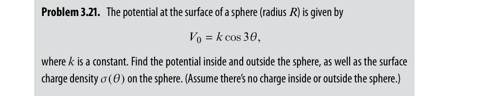
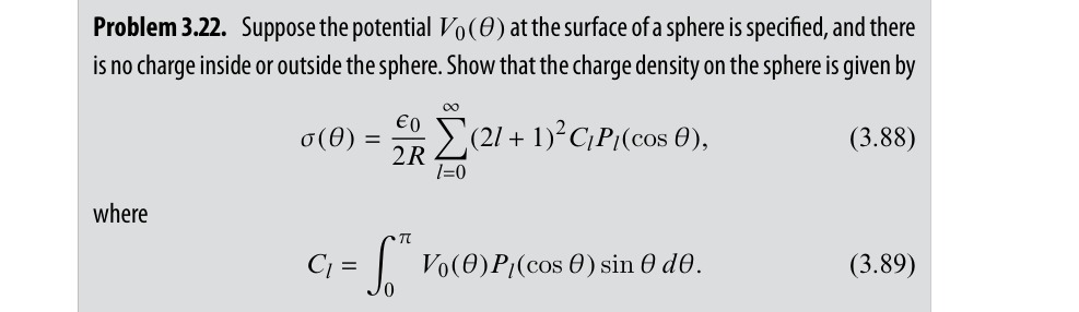
Problem 3.22: The potential on the surface of a sphere of radius $R$ is given by $V_0(\theta) = V_0 \cos(3\theta)$. Find the potential inside and outside the sphere.
習題 3.22:半徑為 $R$ 的球面給定電位為 $V_0(\theta) = V_0\cos(3\theta)$。求球內與球外之電位分佈。
球內電位:$V_{\text{in}}(r, \theta) = \sum_{l=0}^\infty A_l r^l P_l(\cos\theta)$
球外電位:$V_{\text{out}}(r, \theta) = \sum_{l=0}^\infty \frac{B_l}{r^{l+1}} P_l(\cos\theta)$
邊界連續性($r = R$):$V_{\text{in}}(R, \theta) = V_{\text{out}}(R, \theta) \implies B_l = A_l R^{2l+1}$。
電場法向躍變條件:
$$\left. \frac{\partial V_{\text{out}}}{\partial r} \right|_{r=R} - \left. \frac{\partial V_{\text{in}}}{\partial r} \right|_{r=R} = -\frac{\sigma}{\epsilon_0} = -\frac{k}{\epsilon_0}\cos\theta = -\frac{k}{\epsilon_0} P_1(\cos\theta)$$代入微商項:
$$\sum_{l=0}^\infty \left[ -(l+1)\frac{B_l}{R^{l+2}} - l A_l R^{l-1} \right] P_l(\cos\theta) = -\sum_{l=0}^\infty (2l + 1) A_l R^{l-1} P_l(\cos\theta)$$比對 $l=1$ 項:$-(2(1) + 1) A_1 R^0 = -\frac{k}{\epsilon_0} \implies A_1 = \frac{k}{3\epsilon_0}$(其餘階數全為 0)。$B_1 = A_1 R^3 = \frac{k R^3}{3\epsilon_0}$。
物理亮點:球殼內部為均勻電場 $\mathbf{E}_{\text{in}} = -\frac{k}{3\epsilon_0}\hat{\mathbf{z}}$!球外則為純電偶極場!
利用三倍角公式:$\cos(3\theta) = 4\cos^3\theta - 3\cos\theta$。
對照勒壤得多項式:$P_1(x) = x$,$P_3(x) = \frac{1}{2}(5x^3 - 3x) \implies x^3 = \frac{2}{5}P_3(x) + \frac{3}{5}P_1(x)$。
代入得:$\cos(3\theta) = 4\left[ \frac{2}{5}P_3 + \frac{3}{5}P_1 \right] - 3P_1 = \frac{8}{5}P_3(\cos\theta) - \frac{3}{5}P_1(\cos\theta)$。
由邊界條件 $V(R, \theta) = V_0\left[ \frac{8}{5}P_3 - \frac{3}{5}P_1 \right]$,直接寫出係數:
線性電四極子 (Linear Quadrupole) 遠距多極電位展開
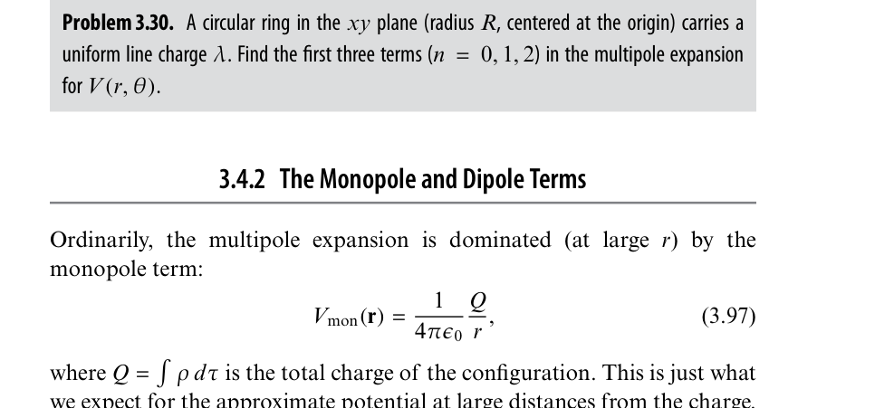
1. 單極項(Monopole Term):
$$Q_{\text{mono}} = \sum q_i = (+q) + (-2q) + (+q) = 0 \implies V_{\text{mono}} = 0$$2. 偶極矩(Dipole Moment):
$$\mathbf{p} = \sum q_i \mathbf{r}_i' = q(d\hat{\mathbf{z}}) + (-2q)(0) + q(-d\hat{\mathbf{z}}) = \mathbf{0} \implies V_{\text{dip}} = 0$$單極矩與偶極矩均為零!故最低非零項必為四極項(Quadrupole Term, $n = 2$)!
多極展開公式通式:
$$V(\mathbf{r}) = \frac{1}{4\pi\epsilon_0} \sum_{n=0}^\infty \frac{1}{r^{n+1}} \sum_{i} q_i (r_i')^n P_n(\cos\alpha_i)$$對於 $n = 2$:
$$\sum_i q_i (r_i')^2 P_2(\cos\theta_i) = q(d)^2 P_2(\cos 0) + (-2q)(0) + q(d)^2 P_2(\cos\pi)$$由於 $\cos 0 = 1, \cos\pi = -1$,且 $P_2(1) = P_2(-1) = 1$:
$$\sum = q d^2 (1) + 0 + q d^2 (1) = 2 q d^2$$因此在場點 $(r, \theta)$ 處,由勒壤得多項式 $P_2(\cos\theta) = \frac{1}{2}(3\cos^2\theta - 1)$:
電四極子電位以 $1/r^3$ 速率衰減,角分佈具有 $(3\cos^2\theta - 1)$ 的四極特徵!